
2
Tutorials Copyright Notice
Copyright © 2002-2015 WhereScape Software Limited. All rights reserved. This document may be
redistributed in its entirety and in this electronic or printed form only without permission; all other
uses of this document and the information it contains require the explicit written permission of
WhereScape Software limited.
Due to continued product development this information may change without notice. WhereScape
Software Limited does not warrant that this document is error-free.
Trademarks
WhereScape and WhereScape RED are trademarks or registered trademarks of WhereScape Software
Limited. Other brands or product names are trademarks or registered trademarks of their respective
companies.
WhereScape USA, Inc
1915 NW AmberGlen Parkway
Suite 400, Beaverton
Oregon 97006
United States
T: 503-466-3979
F: 503-466-3978
WhereScape Limited
P.O.Box 56569, Auckland 1446
Level 3, WhereScape Towers
38 Wyndham Street
Auckland 1010, New Zealand
T: +64-9-358-5678
T: US toll free 1-877-237-3980
F: +64-9-358-5679
WhereScape Asia Pte. Ltd
300 Tampines Avenue 5
#09-02 Singapore 529653
T: +65-6679-5728
WhereScape Europe
Reading Enterprise Centre
Earley Gate, Whiteknights Rd
Reading RG6 6BU
United Kingdom
T: +44-118-914-4509
F: +44-118-914-4508
ii
TABLE OF CONTENTS
Tutorial 1 Basic Star Schema Fact Table 1
1.1 Purpose and Roadmap 2
1.2 The First Step 5
1.3 Repository Defaults 9
1.4 Tablespace (FileGroup) Defaults 11
1.5 Table Name Defaults 13
1.6 Creating a Connection 14
1.7 Loading Source Tables 21
1.8 Building Dimensions 32
1.9 Creating Dimension Views 41
1.10 Defining the Staging Table 45
1.11 Including Dimension Links 49
1.12 Creating a Fact Table 58
1.13 Switching to Diagrammatic View 62
1.14 Producing Documentation 65
1.15 Data Store Objects (Optional) 68
Tutorial 2 Rollup Fact Tables, ASCII File Loads, Aggregates 73
2.1 Purpose and Roadmap 74
2.2 Creating a Connection to Windows 77
2.3 Loading Tables from Flat Files 81
2.4 Creating Stage Tables 87
2.5 Creating Fact Tables 89
2.6 Rollup/Combined Fact Table 91
2.7 Aggregate Tables 95
2.8 Creating a Customer Aggregate 98
Tutorial 3 Scheduling and Dependencies 102
3.1 Purpose and Roadmap 103
3.2 Creating and Scheduling a Job 105
3.3 Adding Tasks 106
3.4 Task Dependencies 109
3.5 Editing a Scheduled Job 111
3.6 Job Results 113
3.7 Diagrammatic View for Jobs 114
Tutorial 4 Complex Dimensions and Hierarchies 116
4.1 Purpose and Roadmap 117
4.2 Creating a Slowly Changing Dimension 118

iii
4.3 Multiple Source Table Dimension 126
4.4 Creating a Dimension Hierarchy 136
Tutorial 5 Analysis Services Cubes 139
5.1 Purpose and Roadmap 140
5.2 Creating an OLAP Cube Object 141
5.3 Adding a Measure Group 170
5.4 Cube Connections for Other Databases 184

1
In This Tutorial
1.1 Purpose and Roadmap.................................................. 2
1.2 The First Step ............................................................... 5
1.3 Repository Defaults ...................................................... 9
1.4 Tablespace (FileGroup) Defaults .................................. 11
1.5 Table Name Defaults .................................................... 13
1.6 Creating a Connection ................................................. 14
1.7 Loading Source Tables ................................................. 21
1.8 Building Dimensions .................................................... 32
1.9 Creating Dimension Views ........................................... 41
1.10 Defining the Staging Table ........................................ 45
1.11 Including Dimension Links ........................................ 49
1.12 Creating a Fact Table ................................................. 58
1.13 Switching to Diagrammatic View ............................... 62
1.14 Producing Documentation ......................................... 65
1.15 Data Store Objects (Optional) .................................... 68
T u t o r i a l 1
Basic Star Schema Fact Table
2
1.1 Purpose and Roadmap
Purpose
This tutorial is designed to introduce you to the basic objects used by WhereScape RED. At the
end of the tutorial you will have built a simple dimensional analysis area of a data warehouse.
The tutorial will build the star-schema shown below. This star-schema comprises a central fact
table, fact_sales_detail, joined to four dimension tables.
Data will be loaded from tables in another SQL Server database, Oracle schema or DB2 schema.
In the process of creating this star-schema you will learn to create load, stage, fact and dimension
tables. You will also see how data flows from the data source, through the different tables enroute
to its fact or dimension table destination.
3
Tutorial Environment
This tutorial has been completed using Microsoft SQL Server. All of the features illustrated in this
tutorial are available in SQL Server, Oracle and DB2 (unless otherwise stated).
Any differences in usage of WhereScape RED between these databases are highlighted.
Tutorial Roadmap
This tutorial works through a number of steps.
These steps and the relevant section within the chapter are summarized below to assist in
guiding you through the tutorial.
Step in Tutorial
Section
Setup the WhereScape tool
Install WhereScape
Set-up tablespace defaults
Set-up default prefixes for tables
Create connection (to data source)
The First Step
Logging In
Tablespace Defaults
Table Name Defaults
Creating a Connection
Create and load the load tables for
Customer
Product
Order_line
Order_header
Loading Source Tables
Create (and update from load tables) the
following dimension tables
Dim_customer
Dim_product
Building Dimensions
Create dimensions for
Dim_order_date
Dim_ship_date
These are views on the dim_date table
Creating Dimension Views
Create the stage_sales_detail table
Create stage table using columns from
load_order_line and load_order_header
Specify join condition
Include links to the following dimensions
(dim_customer, dim_product,
dim_order_date, dim_ship_date)
Defining the Staging Table
Including Dimension Links
Create the fact_sales_detail table
Creating a Fact Table
4
Step in Tutorial
Section
View the WhereScape generated
documentation
Switching to Diagrammatic View
Producing Documentation
5
1.2 The First Step
The first step
To get started you need to follow the steps in the WhereScape Setup Administrator to create the
required environment.
The basic steps in this process are:
Oracle and IBM DB2 data warehouse
1 Install the WhereScape product suite.
2 Create a database schema for the WhereScape metadata repository.
3 Install the WhereScape metadata repository.
SQL Server data warehouse
1 Install the WhereScape product suite onto a computer.
2 Use the Quick Start option in the Setup Administrator utility to load the metadata and
repository.
NOTE: See the RED Installation Guide (sections 2, 7 - SQL Server, 9 - Oracle and 10 - DB2) for
these procedures.
For Oracle this tutorial assumes source data resides in the wtutorial schema and that the
metadata has been loaded under the dssadm schema which has select access to the tutorial
tables.
For SQL Server it assumes that the data warehouse is in the WslWarehouse database and that the
source data resides in the WslTutorial database.
For DB2 it assumes that the data warehouse is in the WhereScape RED schema.
You are now ready to log on (see "1.2.1 Logging In" on page 6) to the repository you have created.
6
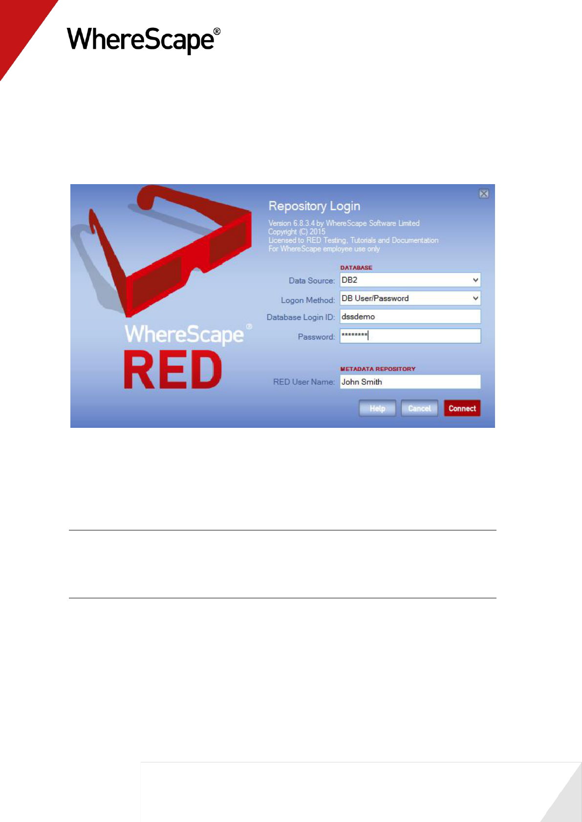
1.2.1 Logging In
Having completed the first step, and using WhereScape RED, you can now log on to the
repository you have created.
To log in:
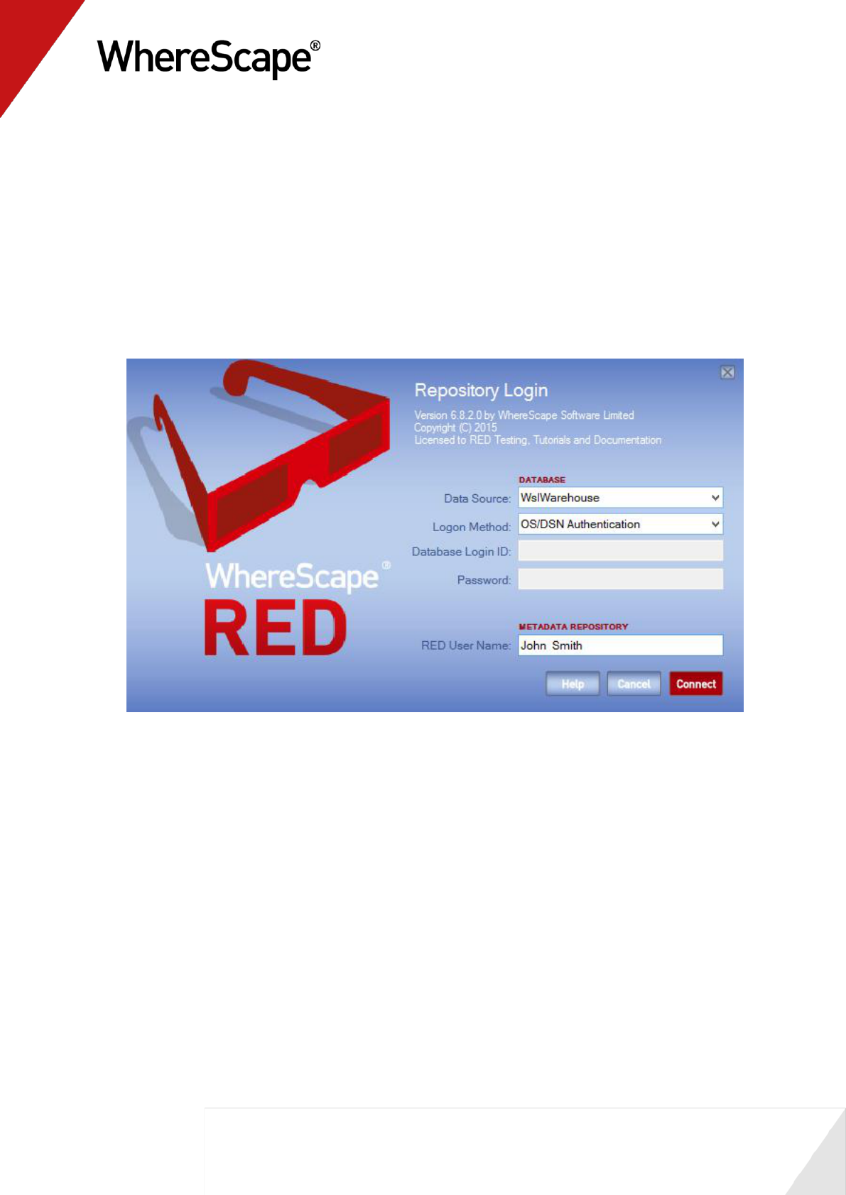
1 Click WhereScape RED from the Start menu. The Access Control screen displays. See sample
screen below:
7
2 For SQL Server, the Data Source, Logon Method and RED Database are the fields required
to logon to the database server if choosing the OS/DSN Authentication Logon Method. If
using the DB/Password Logon Method and a trusted connection is being used enter dbo as the
username.
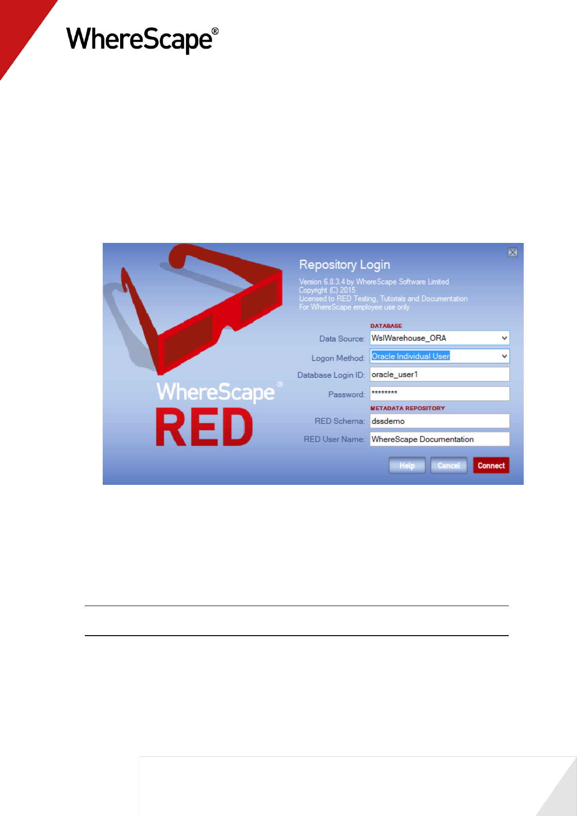
3 For Oracle, select the DB User/Password option on the Logon Method drop-down menu and
enter the Database Login ID and Password. These should be the credentials of the user under
which the metadata repository has been loaded.
4 To log in as a specific individual user, select the Oracle Individual User option from the
Logon Method drop-down menu and enter the user name and password for the user. For more
details about the Oracle Individual User see section 9.3.1 Creating an Oracle Individual
User of the Installation Guide.
5 See Switching Between Databases (see "1.2.2 Switching Between Databases" on page 8) for
details on logging into IBM DB2.
6 The User Name is the name that will be associated with any procedures, tables, etc, and
scheduled jobs that are created from within WhereScape RED. Normally this would be your
full name.
7 Click Connect. The Builder screen displays.
Note: ODBC is the only supported connection method. This connection must have been
established prior to logon. Refer to the RED Installation Guide if no such connection exists.
You are now ready to proceed to the next step where you define the Repository Defaults (see "1.3
Repository Defaults" on page 9). For IBM DB2 authenticated connections see section 1.2.2.
8
1.2.2 Switching Between Databases
The following sample logon screen shows the details entered for IBM DB2 for an operating
system authenticated connection:
For DB2, the Data Source, Database Login ID and Password as well as the Metadata Schema
are those required to logon to the database server.
Select the DB/User Password option from the drop-down menu and enter the Database
Login ID and Password.
NOTE1: A user name and password will be required if operating system authentication is not
being used.
NOTE2: Ignore the Metadata Schema field if connecting to an Oracle or SQL Server repository
after successfully connecting to DB2.

9
1.3 Repository Defaults
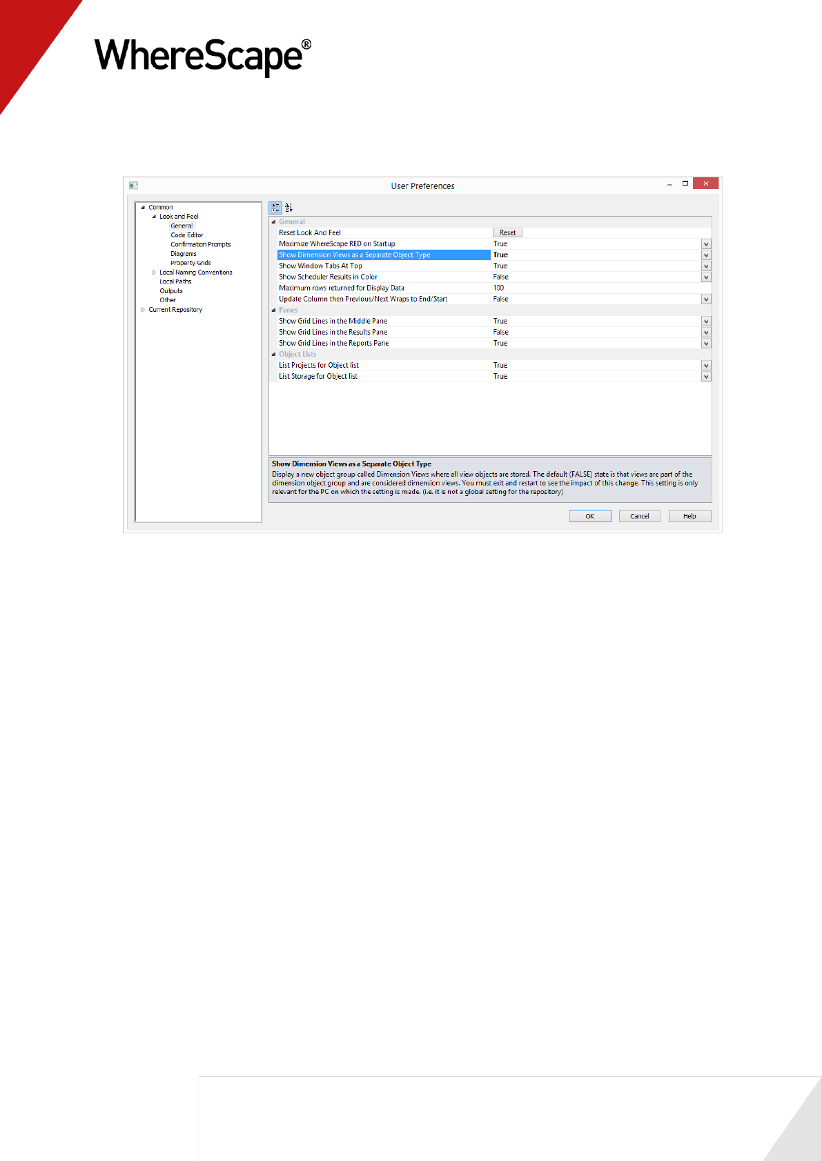
Before you begin to create the data warehouse, you can choose the defaults for the repository.
You can do this from the Tools menu, by either selecting Options or User Preferences.
There is no need to change the defaults for the tutorials.
1 From the Tools menu, select User Preferences.
11
1.4 Tablespace (FileGroup) Defaults
Before you begin to create the data warehouse, you can choose the defaults for the tablespaces
(filegroups for SQL Server).
There is no need to change the defaults for this tutorial.
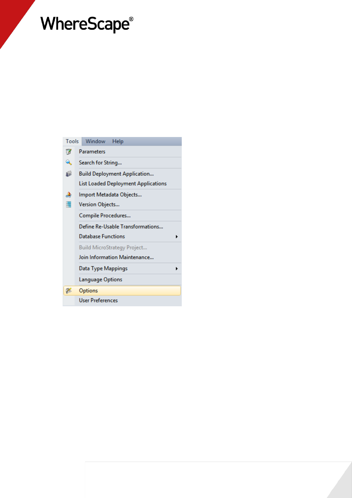
1 From the Tools menu, select Options.
12
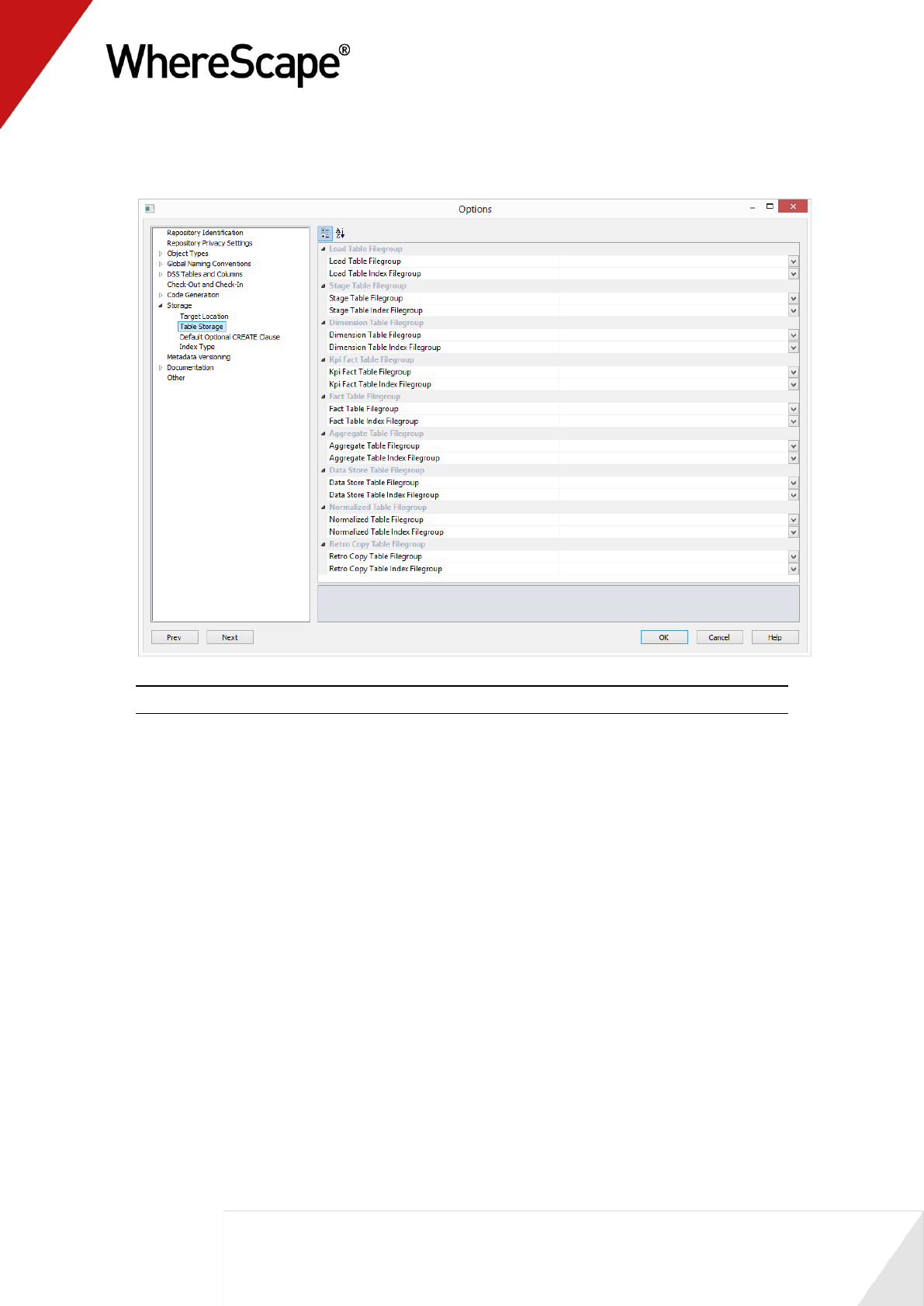
2 Click on Storage and make the appropriate tablespace/filegroup choice for each option.
Click OK.
Note: The default table space or filegroup for the user will be used if no settings are selected.
You are now ready to proceed to the next step where you define the Table Name Defaults (see
"1.5 Table Name Defaults" on page 13).

13
1.5 Table Name Defaults
Before you begin to create the data warehouse, you can choose the defaults for the table names.
There is no need to change the defaults for this tutorial, and the examples given reflect the
default naming convention.
1 From the Tools menu, select User Preferences and then Local Naming Conventions. Alter
the defaults as required.
2 From the Tools menu, select Options and then Global Naming Conventions. Alter the
defaults as required.
3 If no changes are made, the default table names will be:
load_ load tables with data copied from a source system
stage_ tables for manipulating and transforming data prior to publishing
dim_ dimension tables
fact_ fact tables, detail, rollup and snapshot
agg_ aggregate or summary tables built from fact tables
olap_ Analysis Services Olap cubes built from stage or fact tables
You are now ready to proceed to the next step Creating a Connection (see "1.6 Creating a
Connection" on page 14).
14
1.6 Creating a Connection
In order to populate the metadata repository, connections need to be made to the source data.
There must also be a connection to the data warehouse itself.
This section describes how to make two new connections.
Note: The following two connections should have been automatically created. They should
however be validated to ensure they are correct for the environment.
The first connection is to the source system. For Oracle this is the user within your Oracle
database, for SQL Server the database that contains the tutorial tables and for DB2 this is
another schema within your database.
The second connection will be to the data warehouse tables.
TIP: In order to utilize the drag and drop features there must always be a connection to the
data warehouse itself.
How to create a connection
1 Click on and highlight the Connection object group in the left pane. This selects the object
group to be worked on.
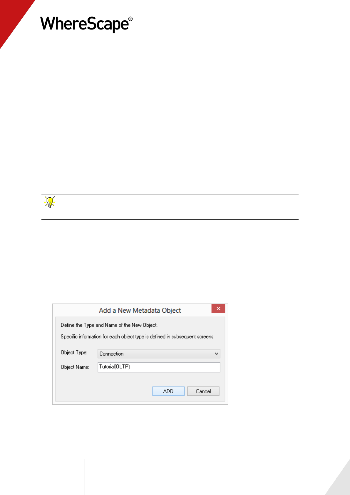
2 Select File|New, or right-click and select New Object. A dialog box displays with the Object
Type defaulted to Connection. Name your connection. In this instance type Tutorial(OLTP)
and click ADD.
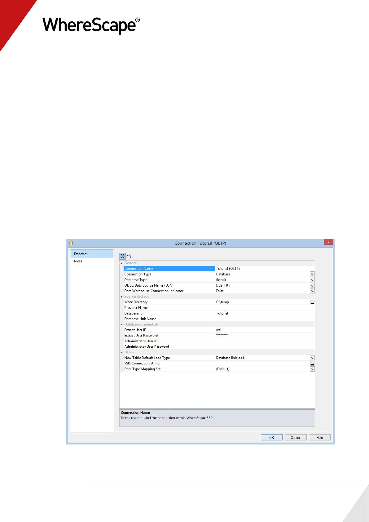
3 A Properties dialog will display.
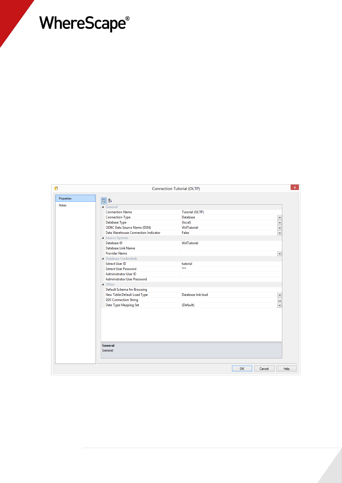
SQL Server:
If running a SQL Server data warehouse then proceed as follows.
In the Properties dialog, complete the details as below, and then select Update:

15
The ODBC Data Source Name (DSN) is the ODBC connection which has been defined to
connect to the database. In this case the ODBC connection to the database that holds the
tutorial tables.
The Provider Name identifies the type of connection that SQL Server will make in the
case of a linked server. In this case it is not required as we are using tutorial tables in a
SQL Server database on the same server.
The Database ID (SID) is the SQL Server database name of the database being connected
to. In this case the SID of the tutorial database.
The Database Link Name is a SQL Server linked server link to connect from the data
warehouse database to the source system database.
Note: This link is only required if the source database is on a different server from the data
warehouse database. For the purposes of this tutorial, the database link ID is not required as
the tutorial data is usually loaded into a database on the same server as the metadata.
16
The Extract User ID and Password are the username and password required to logon to
the tutorial database. If a trusted connection is being used then set the Extract User ID to
"dbo".
The Administrator User ID and Password are the administrator logon to the source
location (tutorial). These can be left blank for the tutorial.
The New Table Default Load Type enables you to set the default load type at connection
level for ODBC and database connections. Set to Database link load.
The SSIS Connection String is a valid SSIS connection string that can be used to connect
to the data source or destination. The Reset button will attempt to construct a valid
connection string from the connection information supplied in the connection details
consisting of the Database ID, Database Link ID (Instance name), Provider Name, Extract
User details. Leave this field blank.
Data Type Mapping Set - XML files have been created to store mappings from one set of
data types to another. Setting this field to "(Default)" will cause RED to automatically
select the relevant mapping set; otherwise you can choose one of the standard mapping
sets from the drop-down list or create a new one.
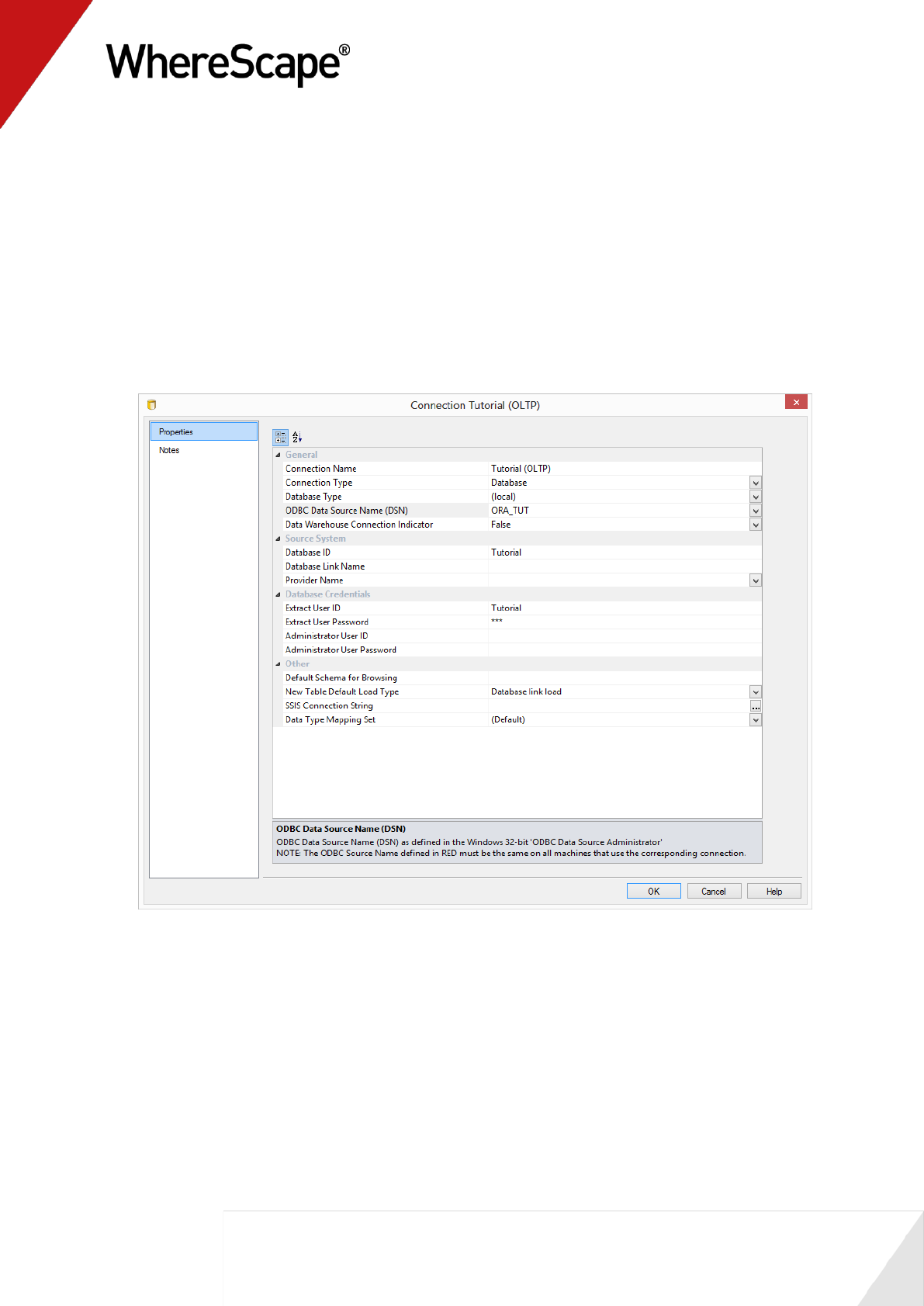
Oracle:
If running an Oracle data warehouse then proceed as follows.
In the Properties dialog, complete the details as below, and then select Update:
17
The ODBC Data Source Name is the ODBC connection which has been defined to
connect to the database. In this case the ODBC connection to the database that holds the
tutorial tables.
The Provider Name identifies the type of connection that Oracle will make in the case of
a linked server. In this case it is not required as we are using tutorial tables in an Oracle
database on the same server.
The Database ID (SID) is the Oracle SID of the database being connected to. In this case
the SID of the tutorial database.
The Database Link Name is an Oracle database link to connect from the data warehouse
database to the source system database.
Note: This link is only required if the source database is different to the data warehouse
database. For the purposes of this tutorial, the database link ID is not required as the tutorial
data is usually loaded into the same database as the metadata.
18
The Extract User ID and Password are the username and password for the schema where
the source tables reside. For the tutorial this is the user where the tutorial files have been
loaded.
The Administrator User ID and Password are the administrator logon to the source
location (tutorial). These can be left blank for the tutorial.
The New Table Default Load Type enables you to set the default load type at connection
level for ODBC and database connections. Set to Database link load.
Data Type Mapping Set - XML files have been created to store mappings from one set of
data types to another. Setting this field to "(Default)" will cause RED to automatically
select the relevant mapping set; otherwise you can choose one of the standard mapping
sets from the drop-down list or create a new one.
IBM DB2:
If running an IBM DB2 data warehouse then proceed as follows.
In the Properties dialog, complete the details as below, and then select Update:
19
The ODBC Data Source Name is the ODBC connection which has been defined to
connect to the database. In this case the ODBC connection to the database that holds the
tutorial tables.
The Provider Name identifies the type of connection that DB2 will make in the case of a
linked server. In this case it is not required as we are using tutorial tables in a DB2
database on the same server.
The Work directory is not used.
The Database ID (SID) is not used.
The Database Link Name is not used.
The Extract User ID and password are the username and password required to logon to
the tutorial database. If an operating system authenticated connection is being used then
leave the Extract User ID and Password blank.
The Administrator User ID and password are the administrator logon to the source
location (tutorial). These can be left blank for the tutorial.
The New Table Default Load Type enables you to set the default load type at connection
level for ODBC and database connections. Set to Database link load.
Data Type Mapping Set - XML files have been created to store mappings from one set of
data types to another. Setting this field to "(Default)" will cause RED to automatically
select the relevant mapping set; otherwise you can choose one of the standard mapping
sets from the drop-down list or create a new one.

20
4 To confirm that you have connected to the system correctly, select Source Tables from the
Browse menu, or click on one of the browse icons from the main tool bar or right pane tool
bar.
Select the connection you want to view, in this instance Tutorial (OLTP), and click OK.
For SQL Server the schema must be set to dbo. For Oracle the schema should be the
tutorial schema.
A third pane on the right, displays showing the tables contained under the tutorial source
system.
5 Repeat steps 1 through 3 to create the connection for the Data Warehouse.
The Connection name will be Data Warehouse
Enter an extract user id (we have used dssadm) and a password (we have used wsl) for the
metadata repository. For a SQL Server trusted connection set the extract user id to dbo.
You have now created two database connections, one to the source system (Tutorial), and one to
the Data Warehouse.
You are now ready to proceed to the next step - Loading Source Tables (see "1.7 Loading Source
Tables" on page 21).
21
1.7 Loading Source Tables
In this step you will load data from the tutorial source system into load tables in the data
warehouse.
Dragging and dropping from the source system (using the previously defined connection) will
create the metadata. You will then be prompted to create and load the tables which will create
the physical tables in the data warehouse, and then load the data.
TIP: Ensure that your source system is displayed in the right pane, by selecting Source
Tables from the Browse menu, then Tutorial (OLTP) from the Connection List. For SQL
Server the schema must be dbo. For Oracle the schema should be the tutorial schema. Click OK.
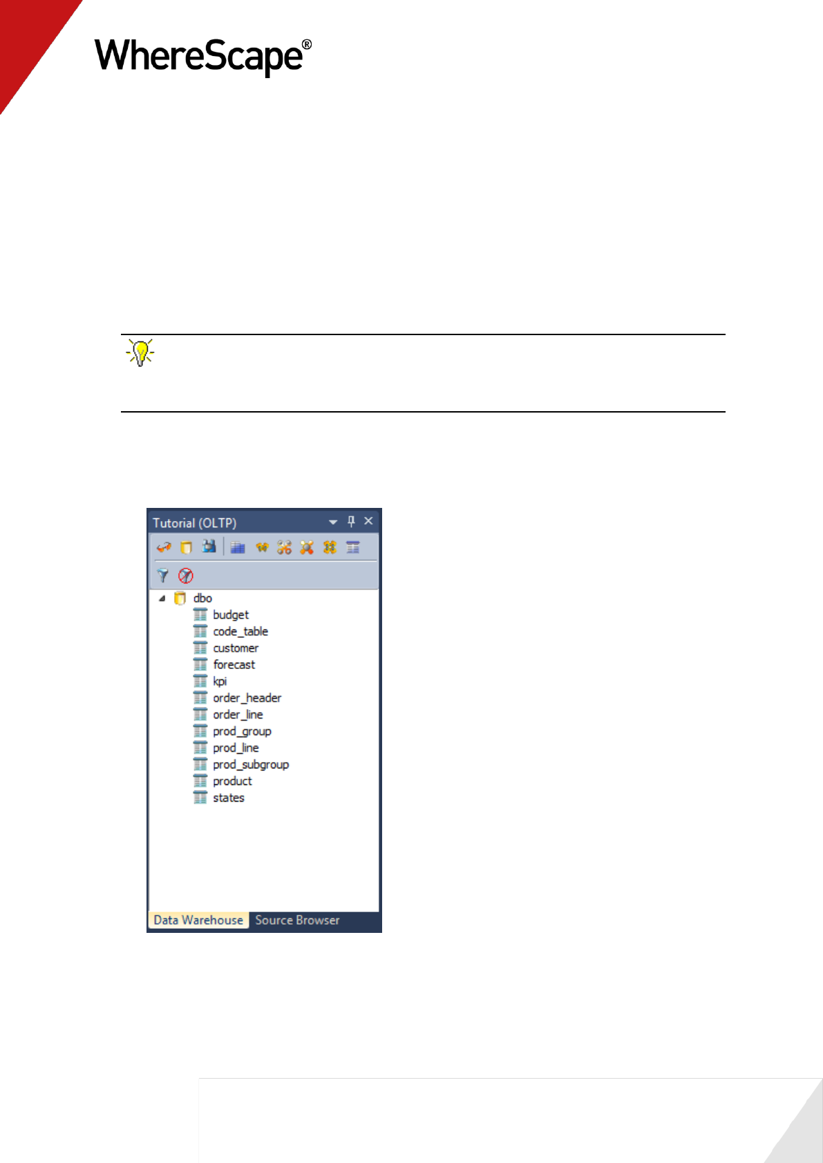
1 Double-click on the Load Table object group on the Object Tree in the left pane. The first
column heading in the middle pane should read Load Table Name.
2 Expand the source table Object Tree in the right pane.
22
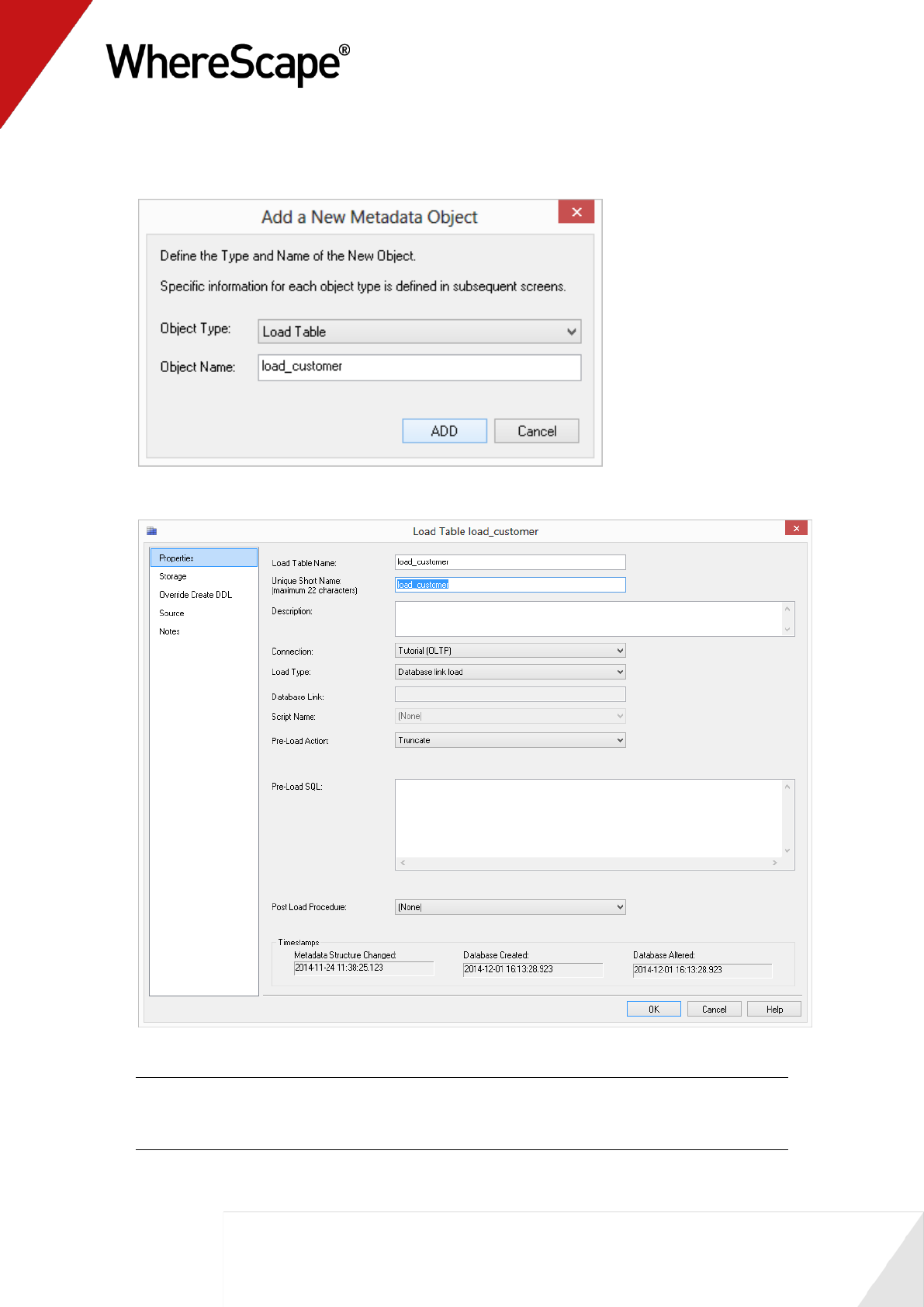
3 Click on customer and drag this table into the middle pane - placing it anywhere in the pane.
A dialog box displays with the name of the object defaulted to load_customer. Click ADD.
4 The following table definition will display. Click OK.
Note1: For the purposes of this tutorial, all the necessary details have been automatically
created. See the Loading Data chapter for explanations of the load parameters.
Note2: In IBM DB2, short names are limited to 12 characters.
23
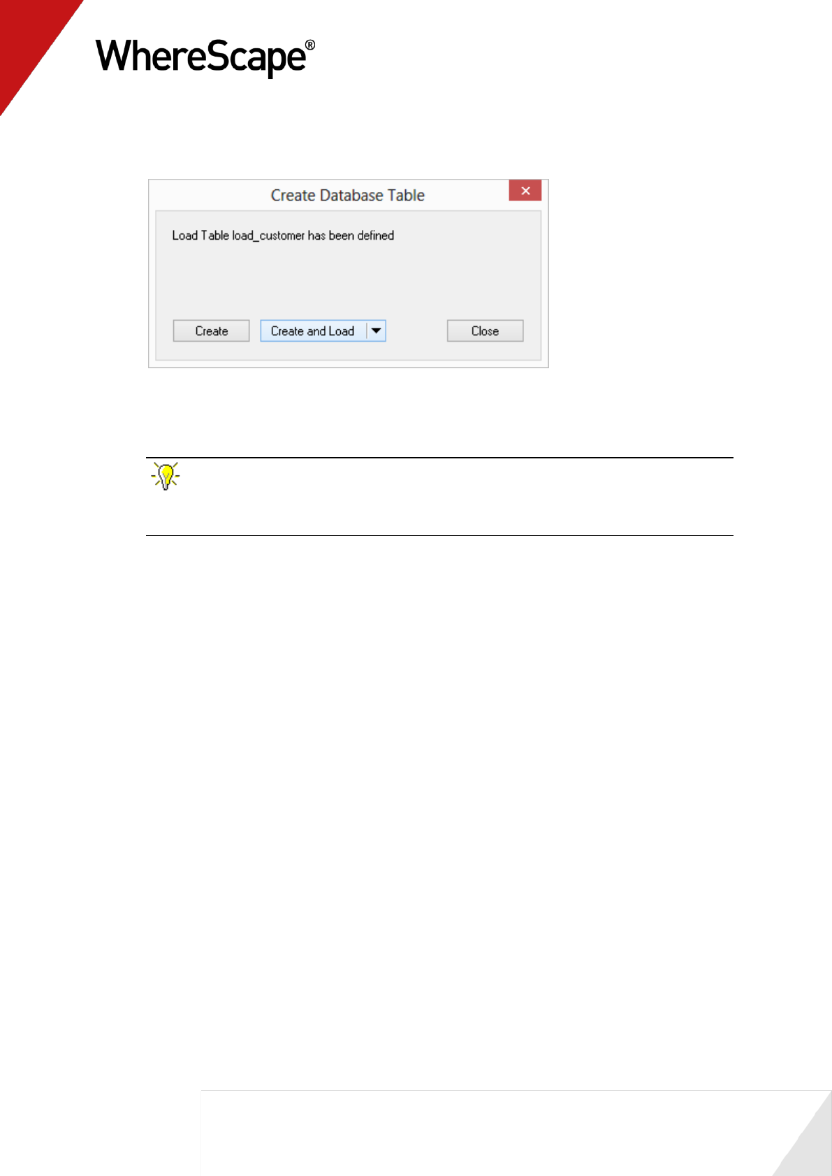
5 A dialog box displays showing that the load table load_customer has been defined and asks if
you want to create and load the table. Click Create and Load.
6 This will create the physical tables in the data warehouse and load the data.
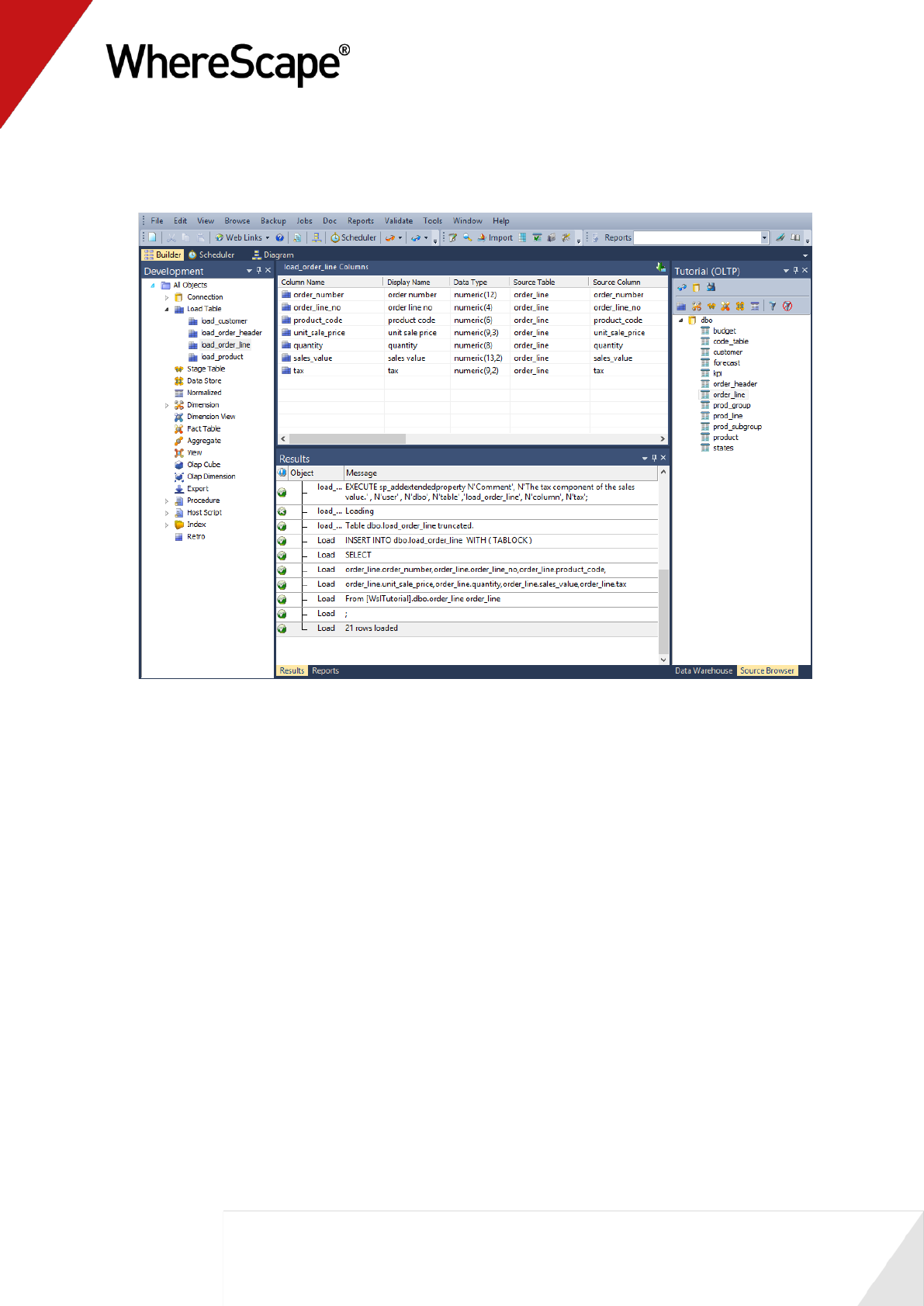
7 Results will be posted in the results pane. Note that the Load Table object group in the left
pane now has a dependent/child.
TIP: Remember to double-click on the left pane Load Table object group between
loading each of the source tables to ensure that you are reassigning the target, rather than
adding to the columns in the middle pane.
8 Repeat this process (steps 2 - 7) for the source tables product, order_header, and order_line.
25
1.7.1 Loading Source Tables using Schemas (Oracle and SQL Server only)
TIP: This an optional/informative tutorial only that has been designed for users that want
to place objects across multiple schemas in WhereScape RED.
RED allows objects to be placed across multiple schemas for Oracle and SQL Server databases.
Before creating any tables using an Oracle source, the RED user needs to be granted a set of
specific privileges.
In SQL Server, the specific shemas will need to be created in the SQL database. The required
Oracle privileges and SQL Server schema instructions are described at the end of this section.
The steps to use schemas in WhereScape RED are:
Ensure the Schema you need exists in Oracle or SQL Server. Create any schema that does not
exist.
Enable Schema use by switching on the Allow Object Schema in Tools>Options.
Add one Target to the Data Warehouse connection in RED for each Schema you intend to
use.
Configure the Data Warehouse connection in RED to browse all required schema by default.
Set the default Target for load tables in Tools>Options.
When you are defining a new table in RED, check and ensure the correct target is set on the
storage tab.
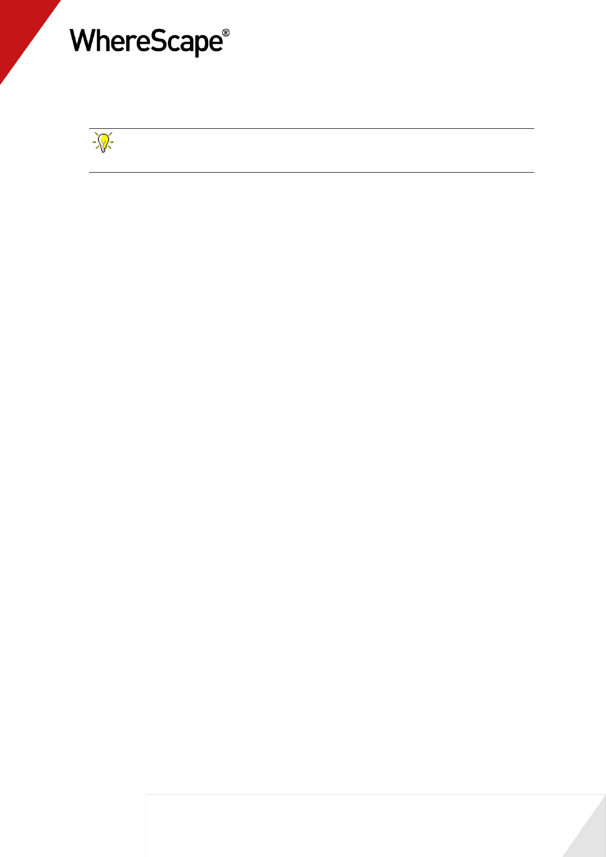
1 After logging in to WhereScape RED, make sure the Allow object Schema option is set in the
Tools->Options->Repository Identification settings.
26
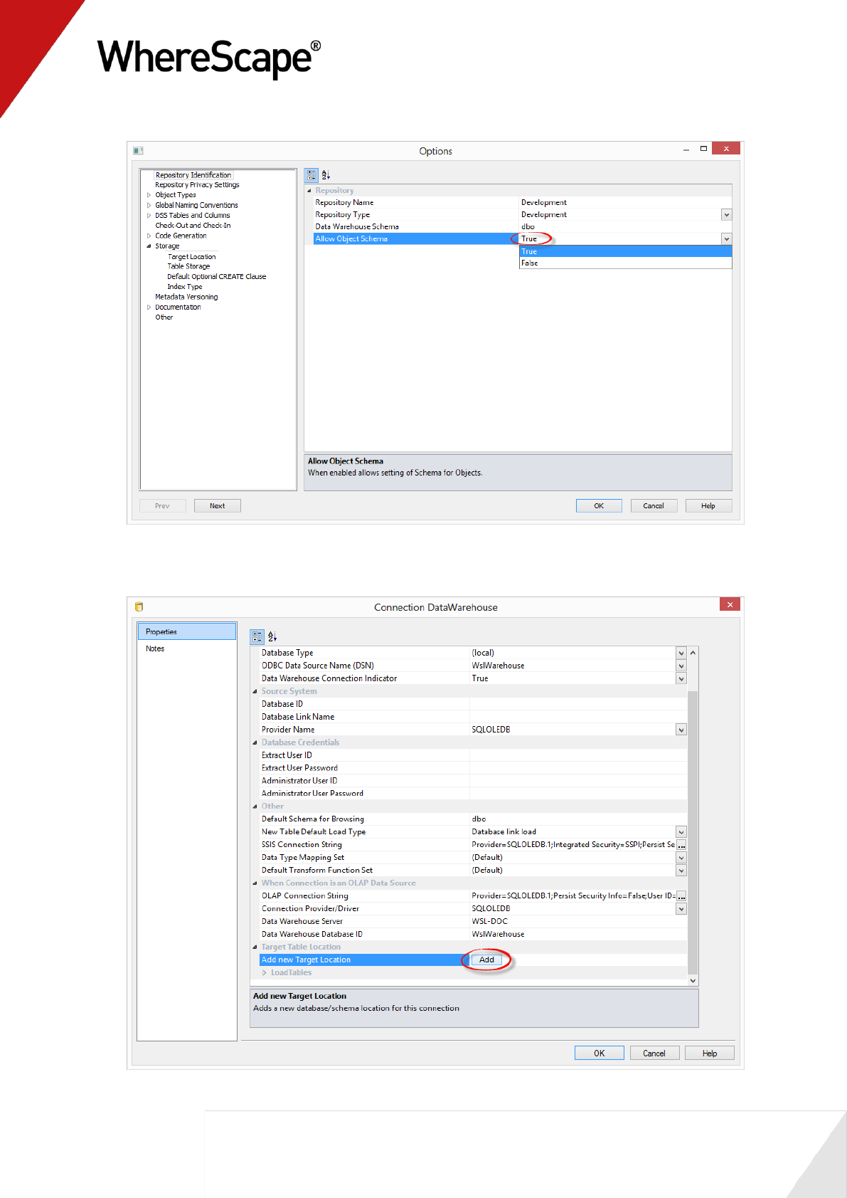
2 Add one Target to the Data Warehouse connection in RED for each Schema you want to use:
Click the Add button to add the required target schemas for this connection.
27
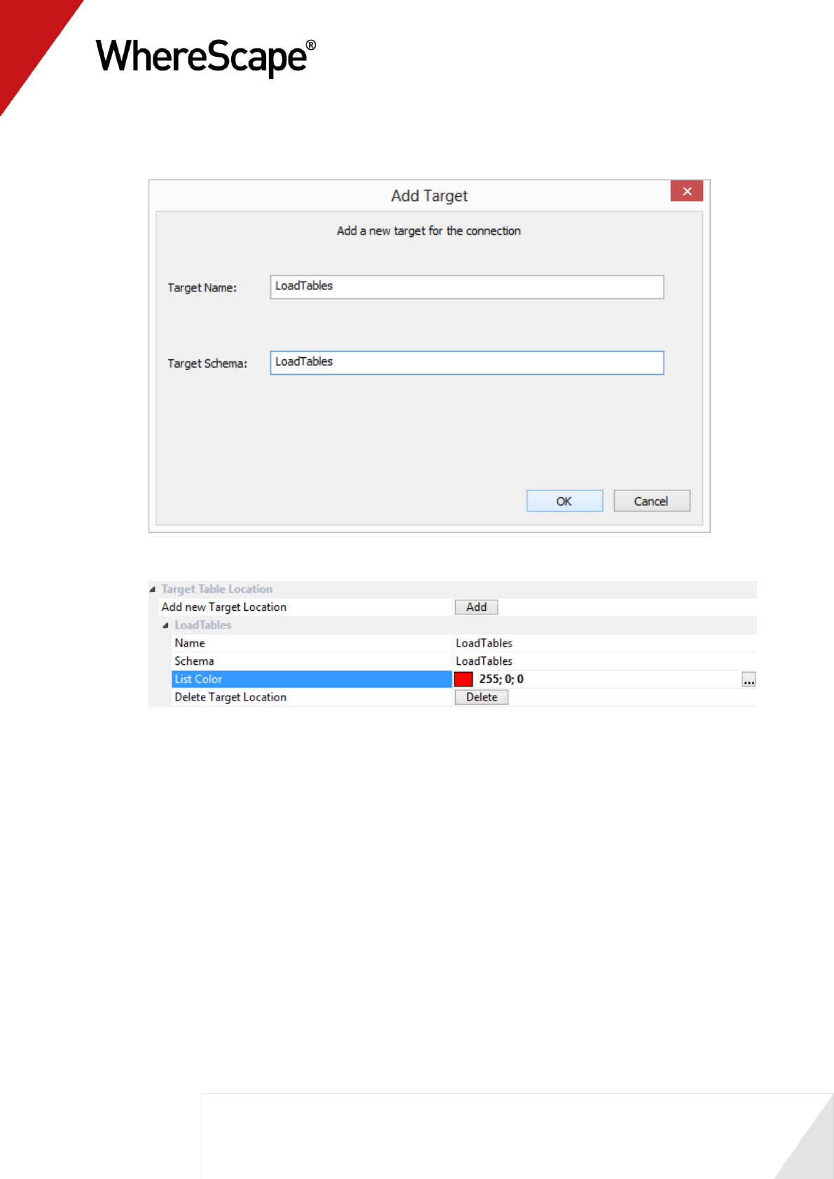
3 Give the new target a name and then enter the target's schema. It is best to set the target
name to the same name as the schema.
4 Expand the target locations to change schema colors or to delete schemas.
28
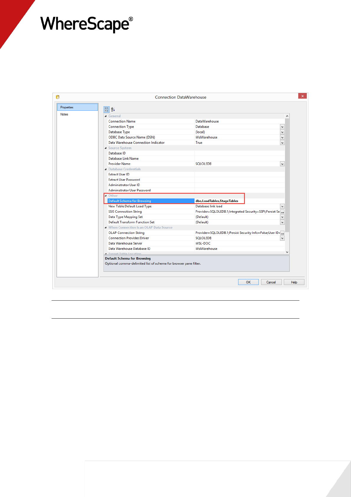
5 Still in the DataWarehouse connection, add the new schemas to the Default Schema for
Browsing field separated by commas.
While browsing this connection, RED will then display a list with all the schemas and
their associated objects on the right-hand browser pane.
NOTE: In SQL Server, you will probably also want to include dbo in this list. Similarly, in
Oracle you will probably also want to include the metadata schema.
29
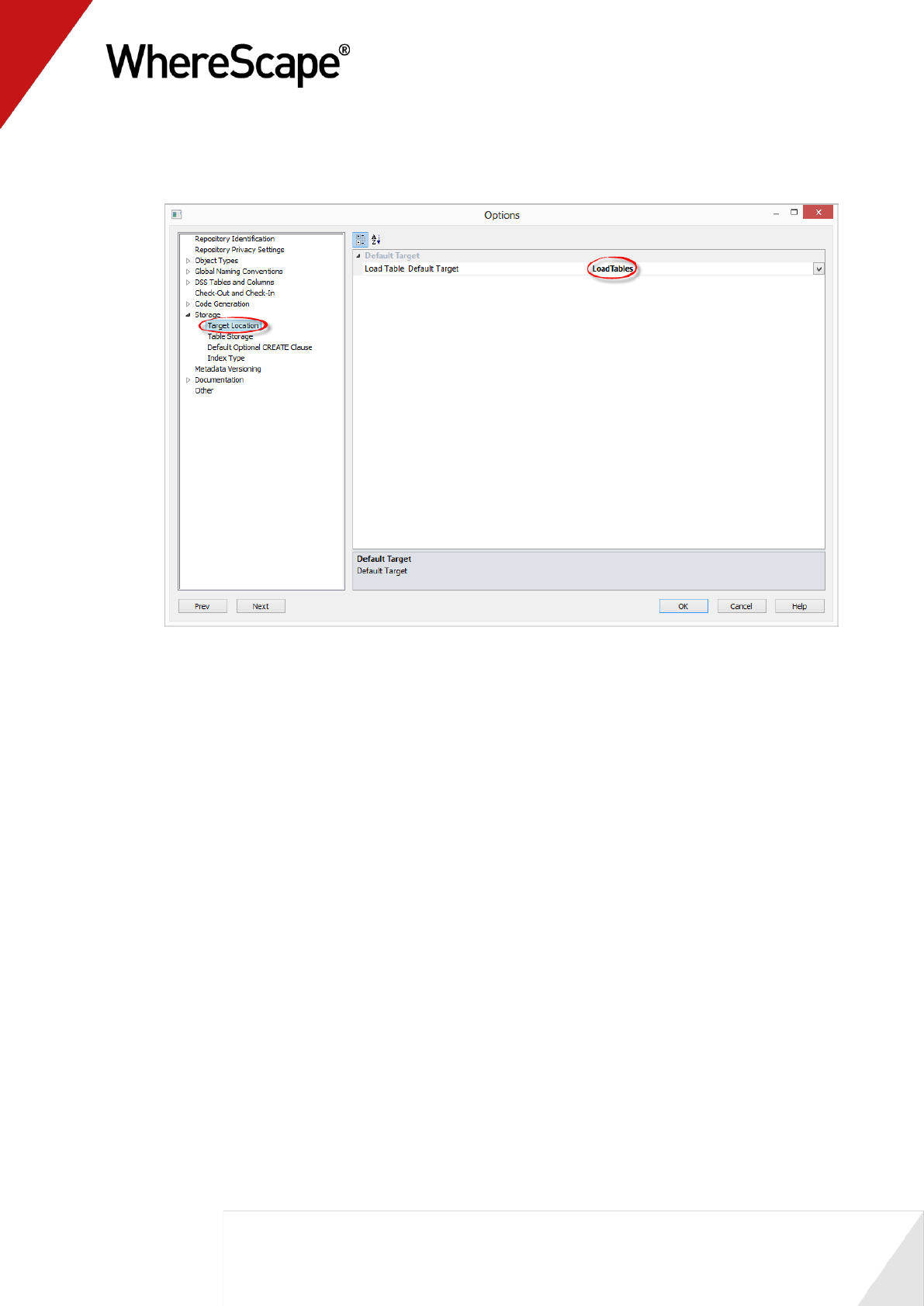
6 You are also able to set the default location for new Load Tables in Tools>Options.
This default target location is only applied when a new load table is created.
30
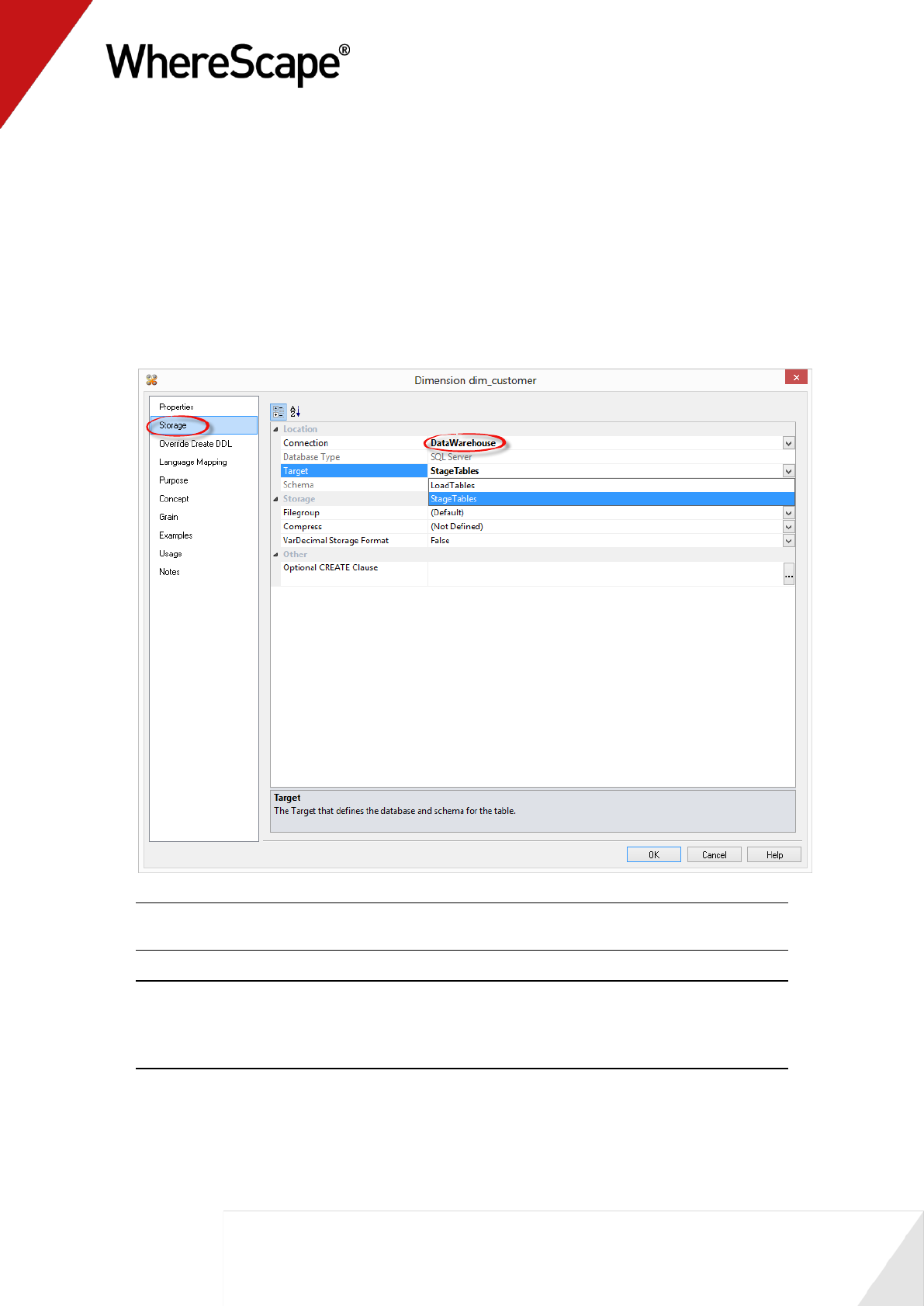
7 When defining a new table in RED, check and ensure the correct target is set on the Storage
tab before creating the table in the database.
A new Load table will have a Target value set by default as defined in step 6. You’re able to
change this as required on each table using the Storage tab of each object's Properties screen.
When using drag and drop, other object types will inherit the default Target value of the
object you create them from. You are also able to change this as required on each table using
the Storage tab of each object's Properties screen.
To locate tables in different schemas, select DataWarehouse from the drop-down menu
and then select the Target schema from the target drop-down menu.
Alternatively, leave this field blank or select (local) for a local table.
WARNING: By default objects will be placed in the source table's schema for table types
other than Load tables.
NOTE: When upgrading from a RED version previous to 6.8.2.0 and moving existing objects
to a target location, all procedures that reference those objects will need to be rebuilt.
Any FROM clauses will also need to be manually regenerated in order for the table references
to be updated to the new [TABLEOWNER] form.
8 To create any of these objects in RED, the RED user will need to be granted a specific set of
privileges in Oracle. For SQL Server, the specific schemas will need to be created in the SQL
database.

31
9 SQL Server
To use object placement across multiple schemas, the required schemas need to be
created in the SQL database.
10 Oracle
To use object placement across multiple schemas in WhereScape RED, the RED user
should be granted the following privileges:
grant select any table to dssdemo;
grant create any view to dssdemo;
grant drop any view to dssdemo;
grant create any table to dssdemo;
grant drop any table to dssdemo;
grant delete any table to dssdemo;
grant insert any table to dssdemo;
grant update any table to dssdemo;
grant alter any table to dssdemo;
grant global query rewrite to dssdemo;
grant create any materialized view to dssdemo;
grant drop any materialized view to dssdemo;
grant alter any materialized view to dssdemo;
grant create any index to dssdemo;
grant drop any index to dssdemo;
grant alter any index to dssdemo;
grant select any sequence to dssdemo;
grant create any sequence to dssdemo;
grant drop any sequence to dssdemo;
grant alter any sequence to dssdemo;
grant analyze any to dssdemo;
32
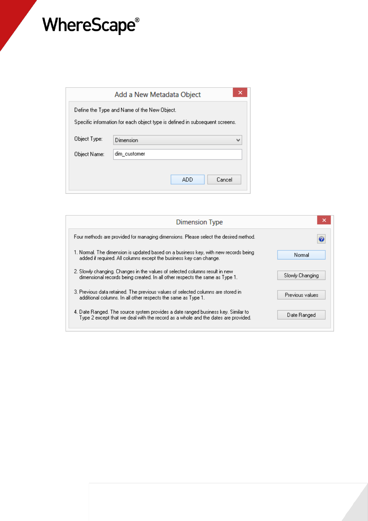
1.8 Building Dimensions
The necessary source tables have been loaded into the data warehouse. Now the dimensions of
the data warehouse can be built. When building dimensions you will be prompted for how you
would like the dimension managed. WhereScape RED generates code for normal, slowly
changing, previous value and date ranged dimensions. You will also be prompted for the business
(or natural) key of the dimension. This is needed so WhereScape RED knows when to add new
dimensional records.
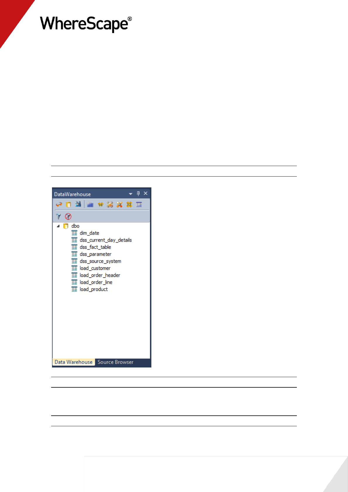
1 Change the right pane view to show the Data Warehouse tables by selecting DataWarehouse
from the Browse menu OR click the tab along the bottom of the source window.
Note: For SQL Server the Data Warehouse schema must be dbo.
Note: From this point onwards, all work will be performed within the data warehouse.
2 Double-click on the Dimension object group in the object tree in the left pane. The first
column of the middle pane now reads Dimension Name.
Note: You will see that some dimensions have already been created for you.
33
3 Click and drag the load_customer table from the data warehouse schema in the right pane
into the middle pane. A dialog box displays defaulting the name of the object to
dim_customer. Click ADD.
4 A dialog box displays asking how you want the dimension managed. Click Normal.
34
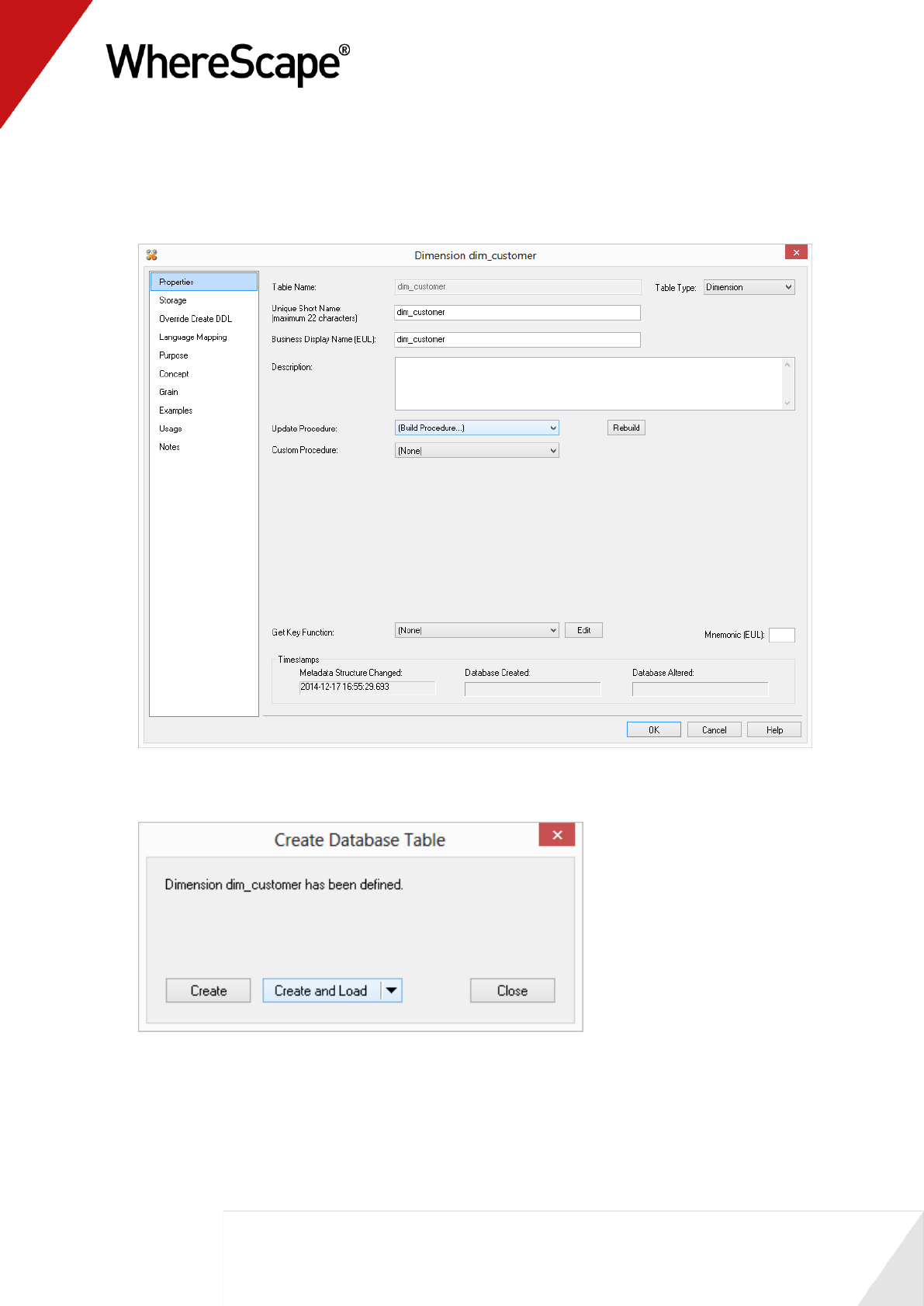
5 A table definition displays with all the necessary defaults completed.
Make one change - Select (Build Procedure...) from the Update Procedure drop-down list
box. This will generate procedures to get surrogate (artificial) keys based on the business
key and to update the dimension. Click OK.
6 A dialog box displays confirming that the dimension table dim_customer has been defined
and asking if you want to create and load the table. Click Create and Load.
35
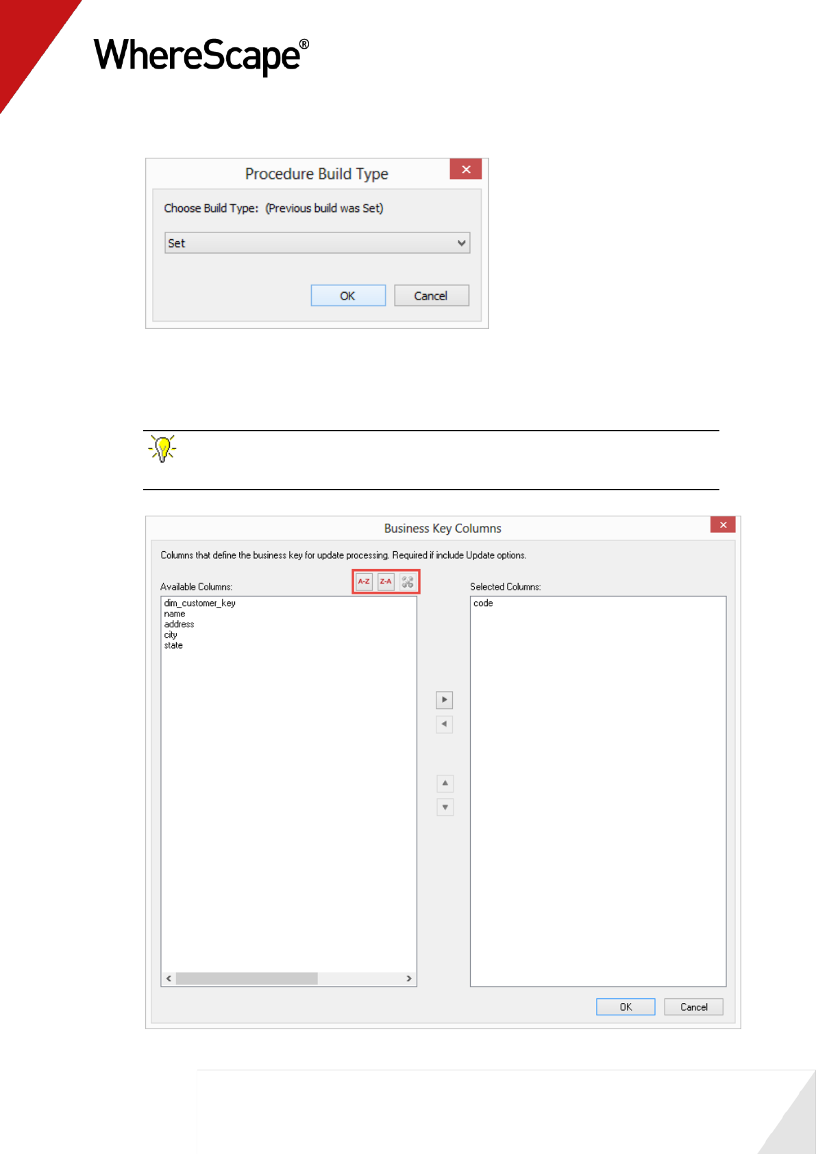
7 A Procedure Build Type dialog will appear. Select Cursor/Set and then click OK.
8 Define the Business Key by clicking on the ellipsis button of the Update Build Options
screen.The business (natural) key is the unique identifier for the dimensional record.
Select code and > (or double-click on code) on the Business Key Column dialog and click OK.
TIP: The toggle sort button button can help to sort Business Key columns into
alphabetic order.
36
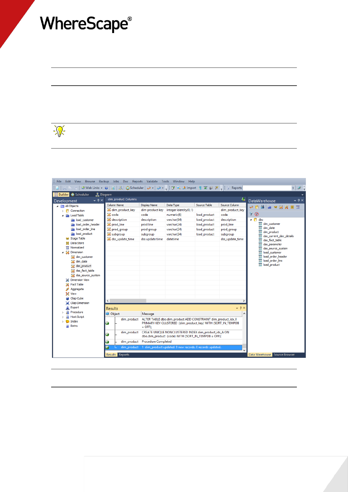
9 The procedure results display and can be reviewed.
NOTE: The Dimension Table object group in the left pane now has added dim_customer as a
dependent/child.
10 Repeat this same process (steps 2 through 9) for the load table load_product. The business
key will be code.
TIP: Remember to double-click on the left pane Dimension Table object group between
loading each of the above dimension tables.
11 Refresh the Data Warehouse pane on the right (F5).
Your screen should look something like this:
Note: Analysis Services does not like name as a column name. For dim_customer it will
therefore be necessary to change the column name from name to cname.
12 Click on dim_customer in the left pane to display the dim_customer columns in the middle
pane.

37
13 When positioned on the column name in the middle pane, right-click and select Properties
from the drop-down menu.
14 Change the column name and business display name from name to cname as shown below.
Click OK.
38
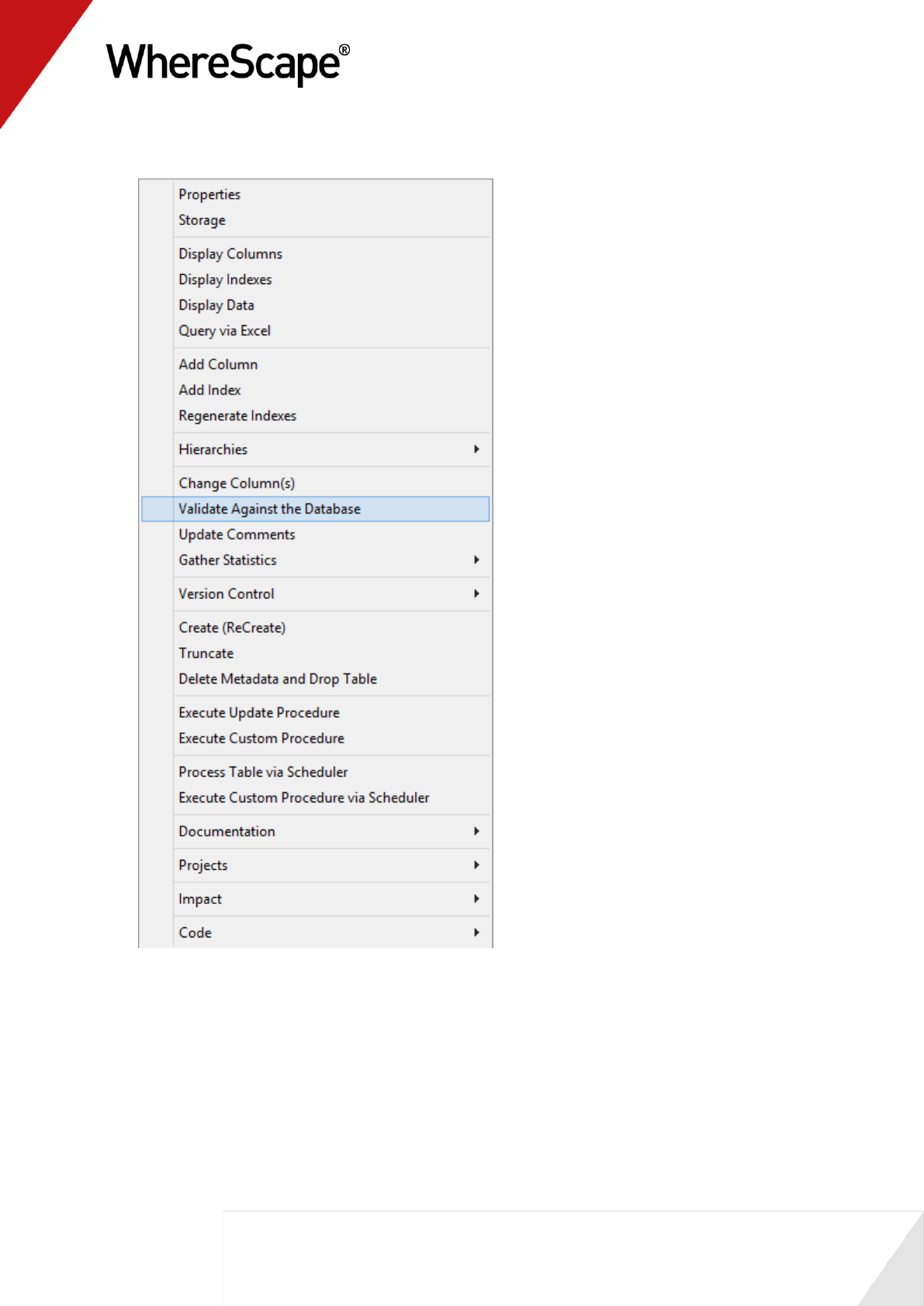
15 Right-click on dim_customer in the left pane and select Validate against the Database.
39
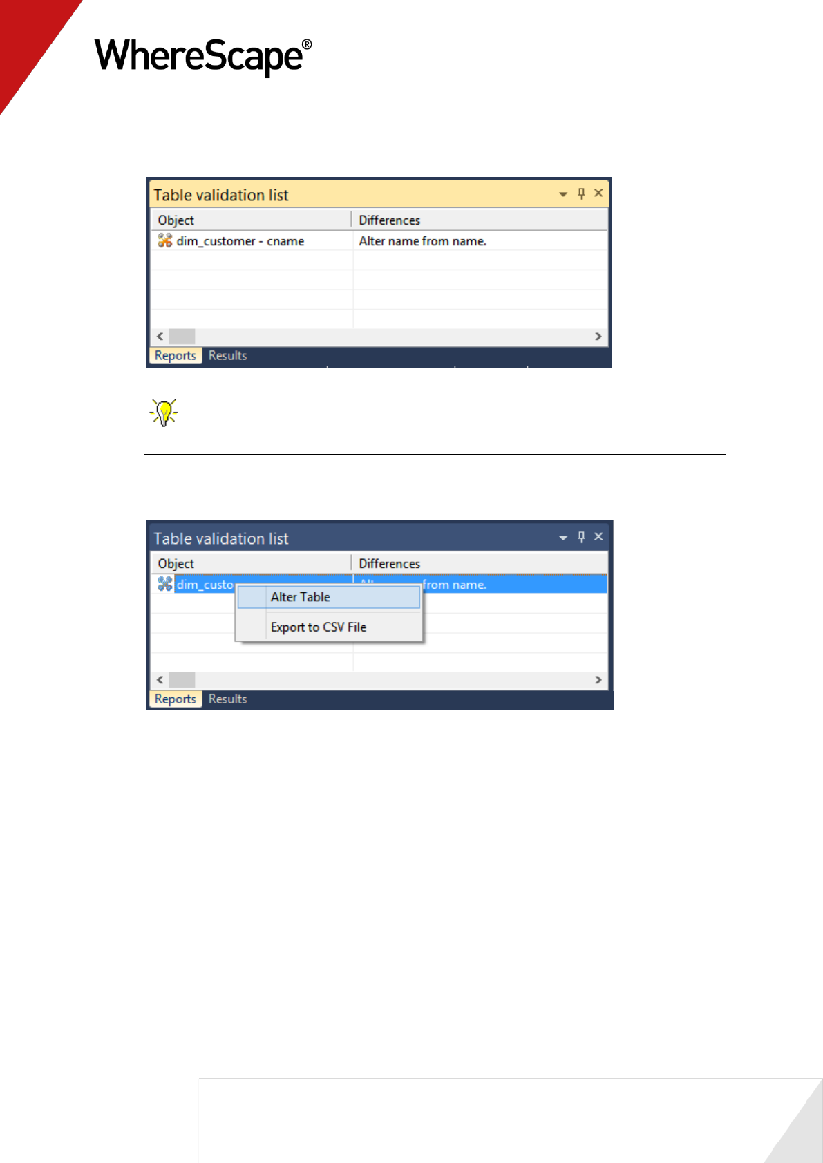
16 The results will show that the metadata has been changed to cname while the column name
in the database is still name.
TIP: You can right click on the dimension name and select Sync Column order with
database to reorder the metadata columns to match the column order in the database table.
17 Right-click on dim_customer in the bottom pane and select Alter table from the drop-down
list.
40
18 A warning dialog will appear, displaying the table and column name to be altered. Select
Alter Table.
19 A dialog will appear confirming that dim_customer has been altered. Click OK.
20 Right-click on the dim_customer object in the left pane and select Properties from the
drop-down menu. Choose the Rebuild button.
21 A Procedure Build Type dialog will appear. Select Cursor and then OK.
22 Leave the Business key as Code and click OK.
23 Right-click on dim_customer in the left pane and select Execute Update Procedure.
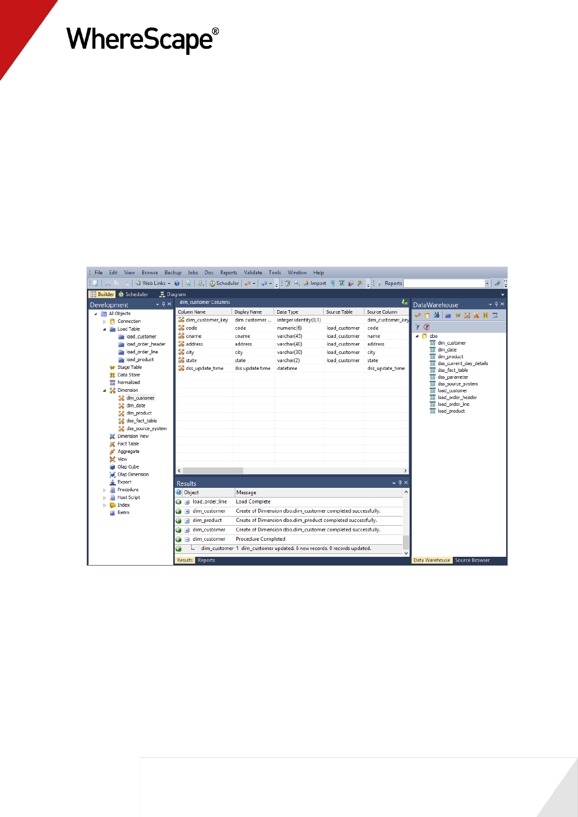
24 Click in the right pane and press F5 to refresh the Data Warehouse table view.
25 Your screen should look something like this:
You are now ready to proceed to the next step - Creating Dimension Views (see "1.9 Creating
Dimension Views" on page 41)
41
1.9 Creating Dimension Views
A dimension view is a database view of a dimension table. It may be a full or partial view. It is
typically used in such cases as date dimensions where multiple date dimensions exist for one fact
table.
In this step you will create dimension views from an existing dimension. In many cases
dimension views are built as part of the end user layer, but creating them in the data warehouse
means they are available regardless of the end user tools used. This process is essentially the
same as creating a dimension, but you are creating a view of an existing dimension, in this
instance, dim_date.
1 After double-clicking on Dimension View in the left pane, click and drag dim_date from the
right pane into the middle pane.
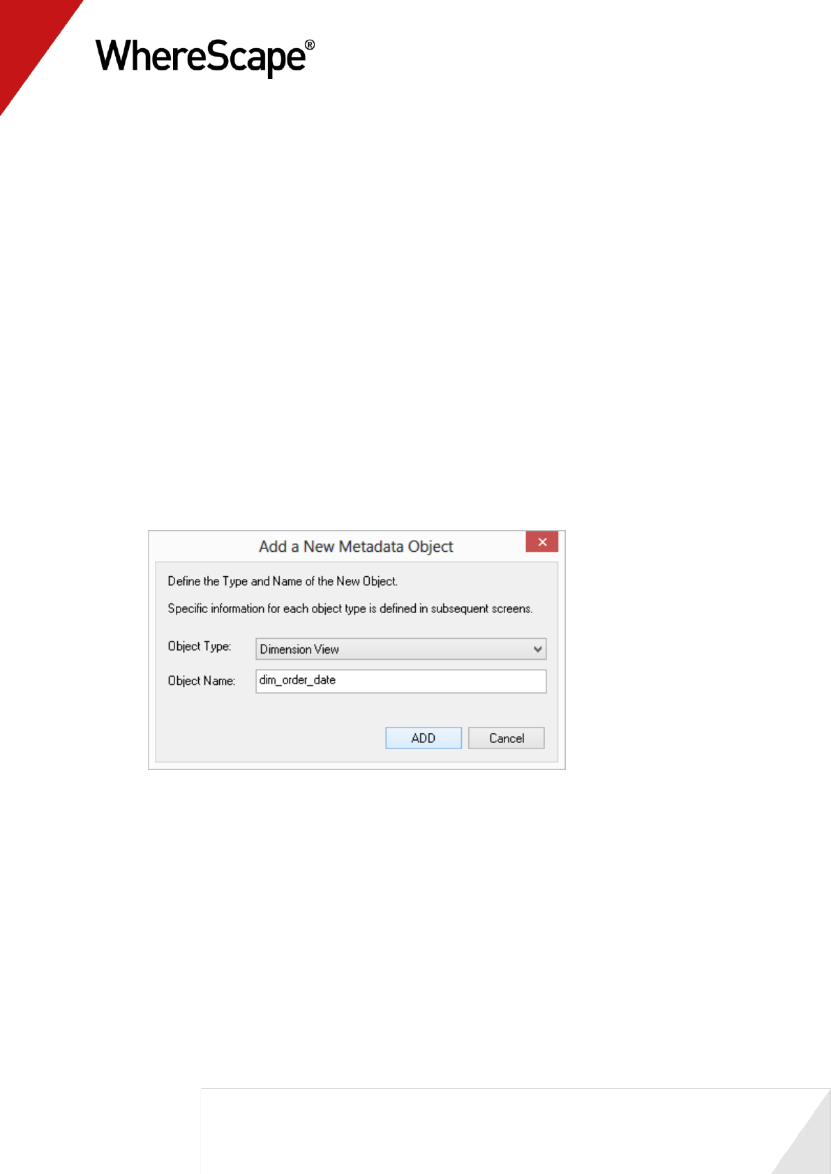
The dialog box that displays defaults the object type to a dimension view, and names the
dimension view dim_date.
Because we want to create two dimension views from the same source, dim_date, we need
to change this dimension view name to one that is more meaningful, specifically
dim_order_date. Make this change and click ADD.
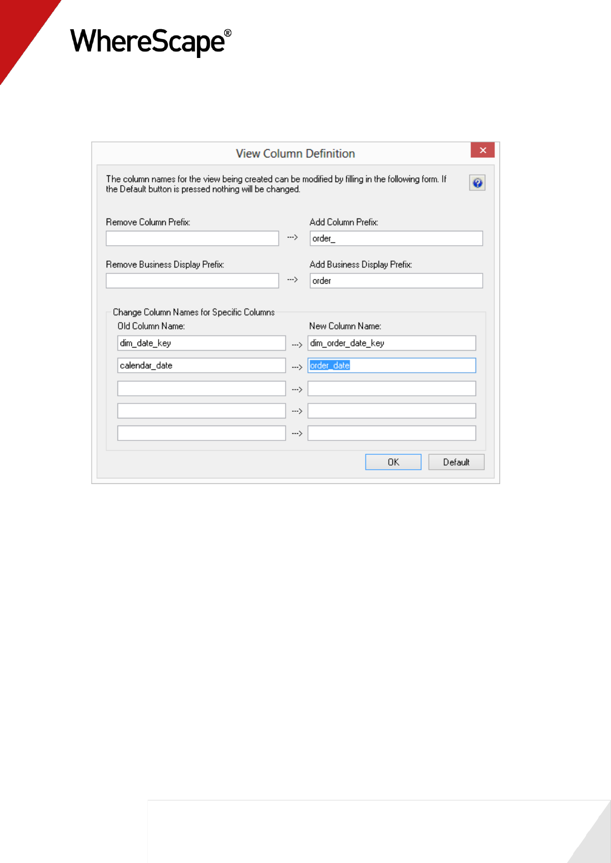
42
2 A dialog box displays to provide a means of re-mapping some of the column names in the
view if required. Rename calendar_date to order_date and click OK.

43
3 The dim_order_date view property defaults have all been completed as necessary so click OK.
4 A dialog box displays indicating that the dimension view dim_order_date has been defined
and asks if you want to create the view now. Select Create View + Function.
5 Click OK on the Business Key dialog.
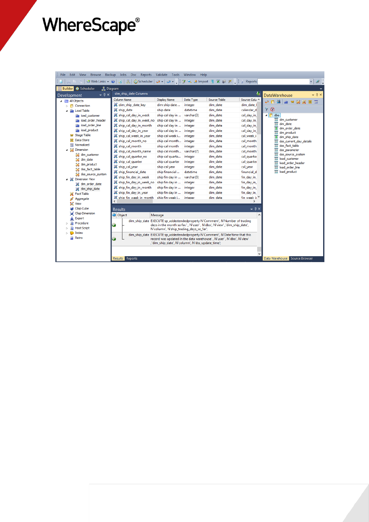
6 Repeat steps (1) to (5) to create the dimension view dim_ship_date.
7 Click in the right pane and press F5 to refresh the Data Warehouse table view in the right
pane.
45
1.10 Defining the Staging Table
In this step you will create a stage table from two load tables. A stage table is used to build the
format of the fact table, and generally contains changed or new data that will be added to the fact
table. As stage tables contain dimensional keys, they should be defined after the dimensions.
Note: The source of data for the stage table will be the load tables load_order_line and
load_order_header.
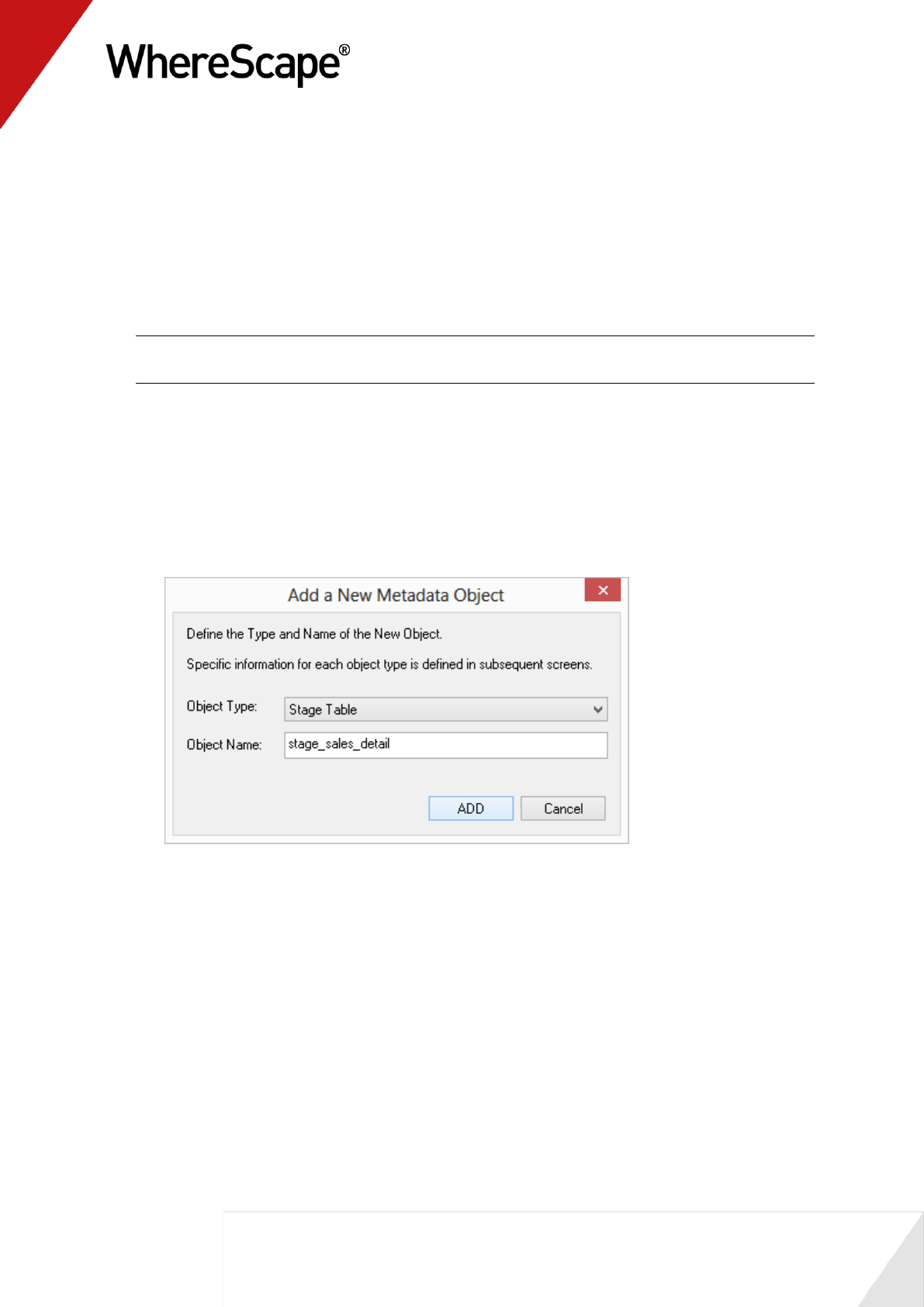
1 Double-click on the Stage Table object group in the object tree in the left pane to create a
stage table target. The first column heading in the middle pane reads Stage Table Name.
2 Click and drag the load_order_line table from the right pane data warehouse schema. Drop it
in the middle pane. A dialog box displays defaulting the name of the object to
stage_order_line. To make it a more meaningful name, change the name of the object to
stage_sales_detail and click ADD.
46
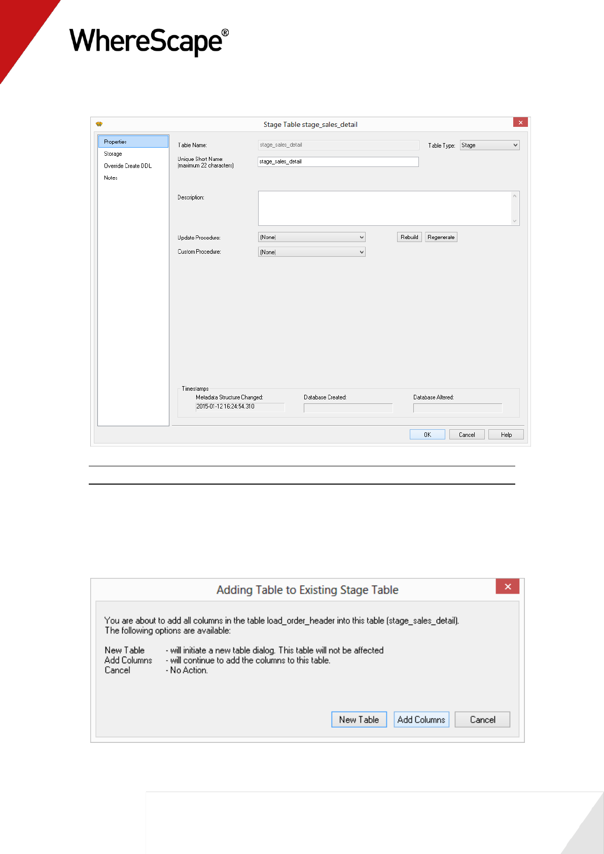
3 A table definition displays with all the necessary defaults completed. Click OK.
Note: The Stage Table object group in the left pane now has a dependent/child.
4 To add the remaining information from the second load table, click on stage_sales_detail in
the left pane. Next drop load_order_header from the right pane into the middle pane.
5 A message is displayed with options to create a "New table" or to "Add columns". Click Add
Columns.
47
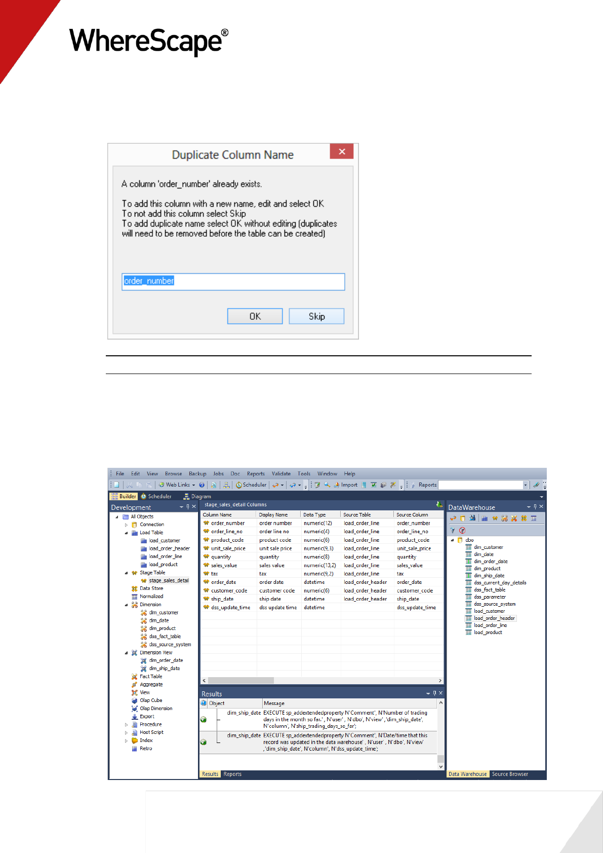
6 WhereScape RED detects duplicated columns. As both load_order_header and
load_order_line have the order number field, the following is displayed. Click Skip to
exclude the second instance of order_number.
Note: If the second instance of order_number is required, then click OK.
7 This combines data from two load tables (load_order_header and load_order_line) into one
stage table. In the middle pane under Source Table, notice the source of each of the columns.
8 Your screen should look something like this:

49
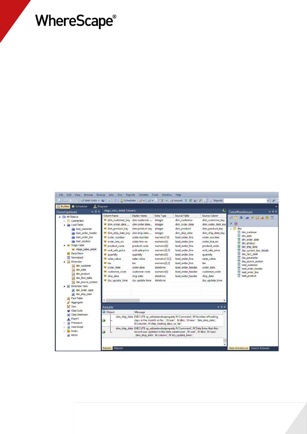
1.11 Including Dimension Links
The dimension links that allow us to create the fact-like star schema now need to be included:
1 In the left pane, click on the stage_sales_detail table in the Stage Table object group. The
middle pane should display the contents of this stage table.
2 Drag each of the following dimensions from the right pane into the stage table in the middle
pane:
dim_customer
dim_order_date
dim_product
dim_ship_date
This adds the dimension keys from each dimension to the stage table. Your WhereScape RED
screen should now look like this:
50
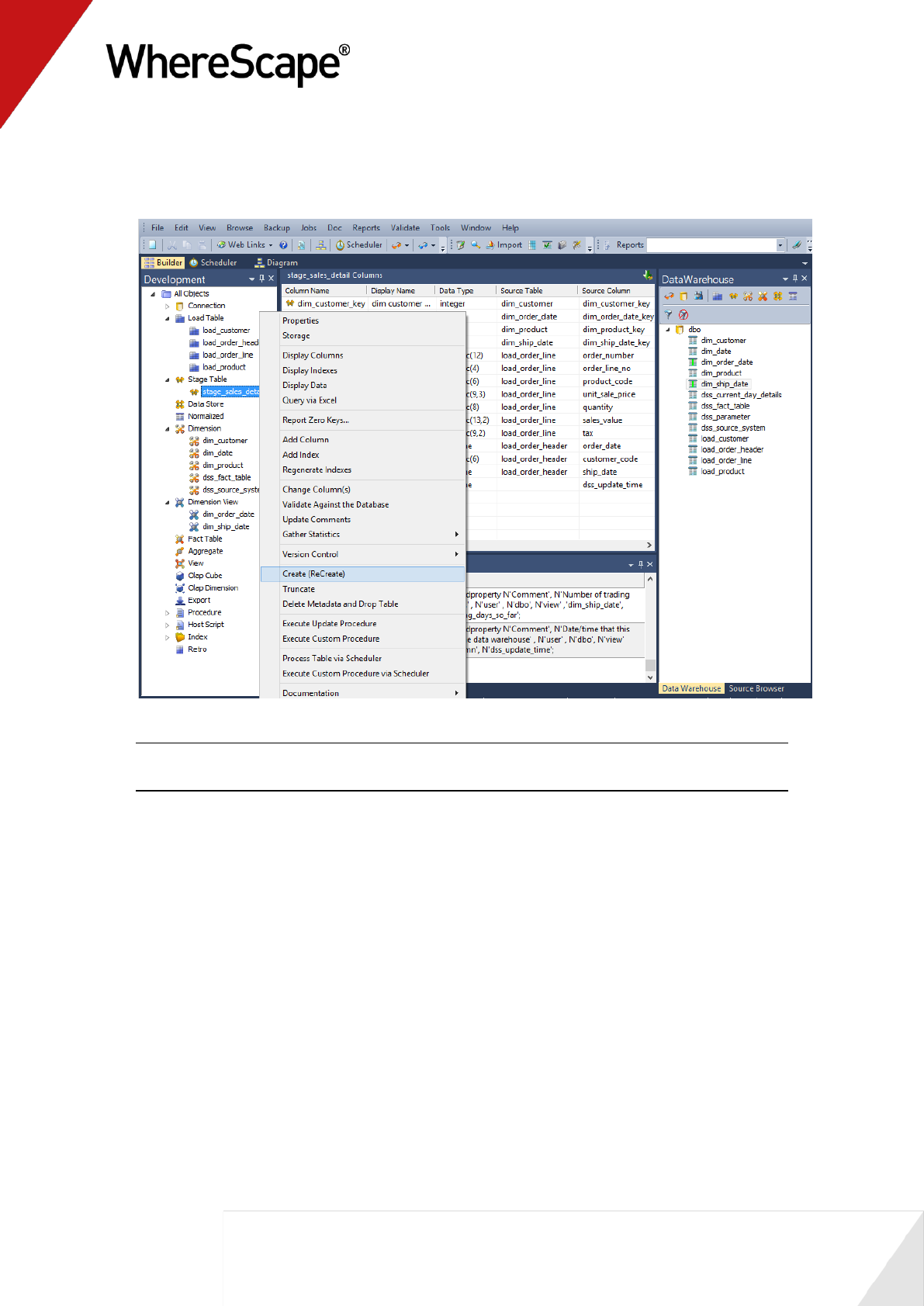
3 The stage table metadata has been defined, but the stage table has not been created. To
create the stage table in the data warehouse, right-click on stage_sales_detail in the left
pane and select Create (ReCreate).
Note: The table must exist in the data warehouse before we can proceed to the next step. If
the table has not been physically created then the procedure in step 5 will fail to compile.
51
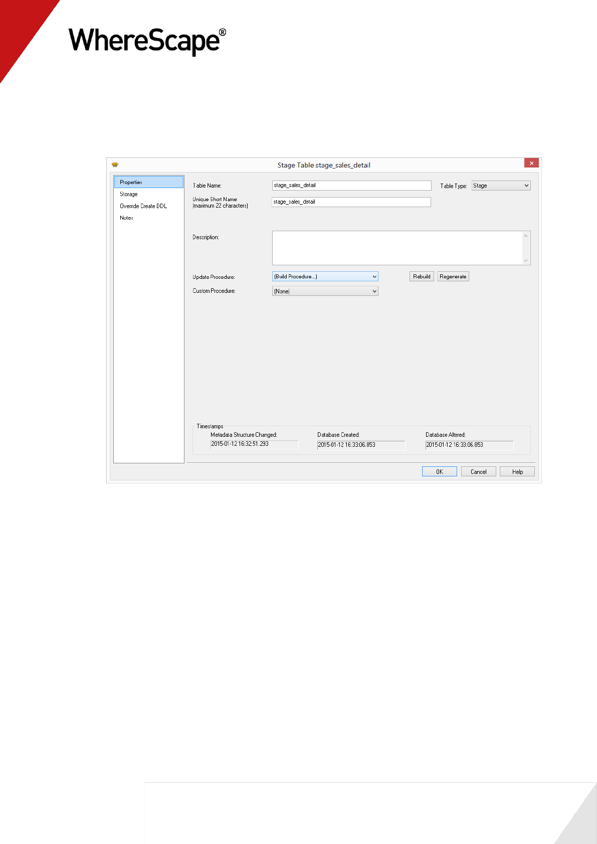
4 Double-click on the stage table to select Properties.
5 Under Update Procedure, choose (Build Procedure...) to create an update stage procedure.
Click OK.
52
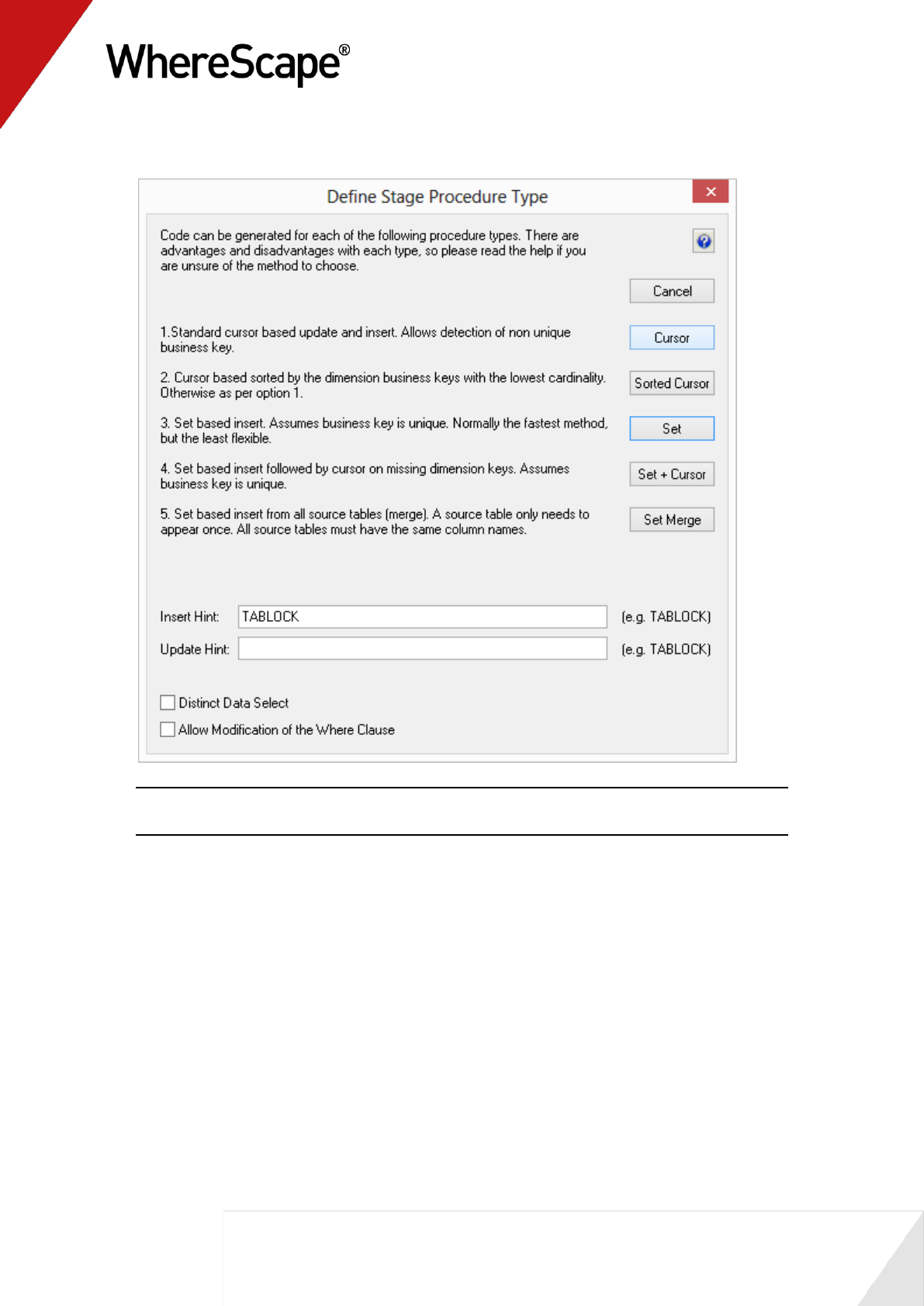
6 Select the Cursor based procedure generation from the stage procedure type dialog box.
Note: When building an Oracle data warehouse, this dialog has an additional option for bulk
bind procedures. See Staging generating the update procedure for more information.
53
7 Click OK on the Parameters dialog.
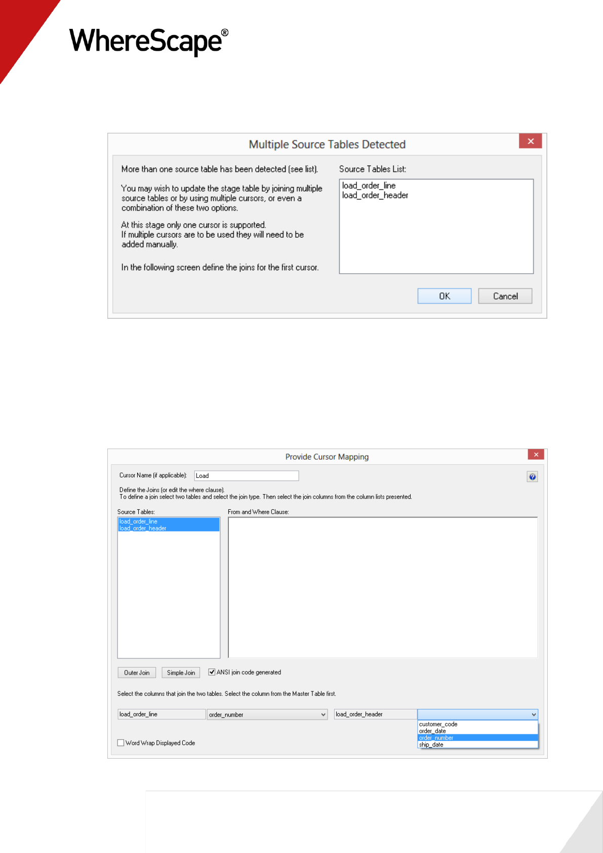
8 A dialog box will display indicating that multiple source tables have been detected. Click OK.
9 Highlight the source tables load_order_line and load_order_header which are to be joined
by order_number.
With the two tables highlighted click Outer Join. See the chapter on Staging data for an
explanation of the join types and options.
Select order number from the load_order_line empty drop-down list box at the bottom
of the screen. Then select order number from the load_order_header drop-down list box.
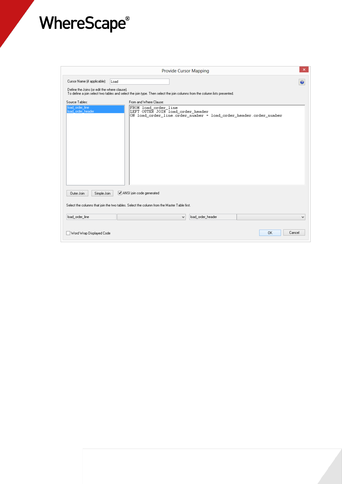
54
This will create a join statement in the right window. Click OK.
55
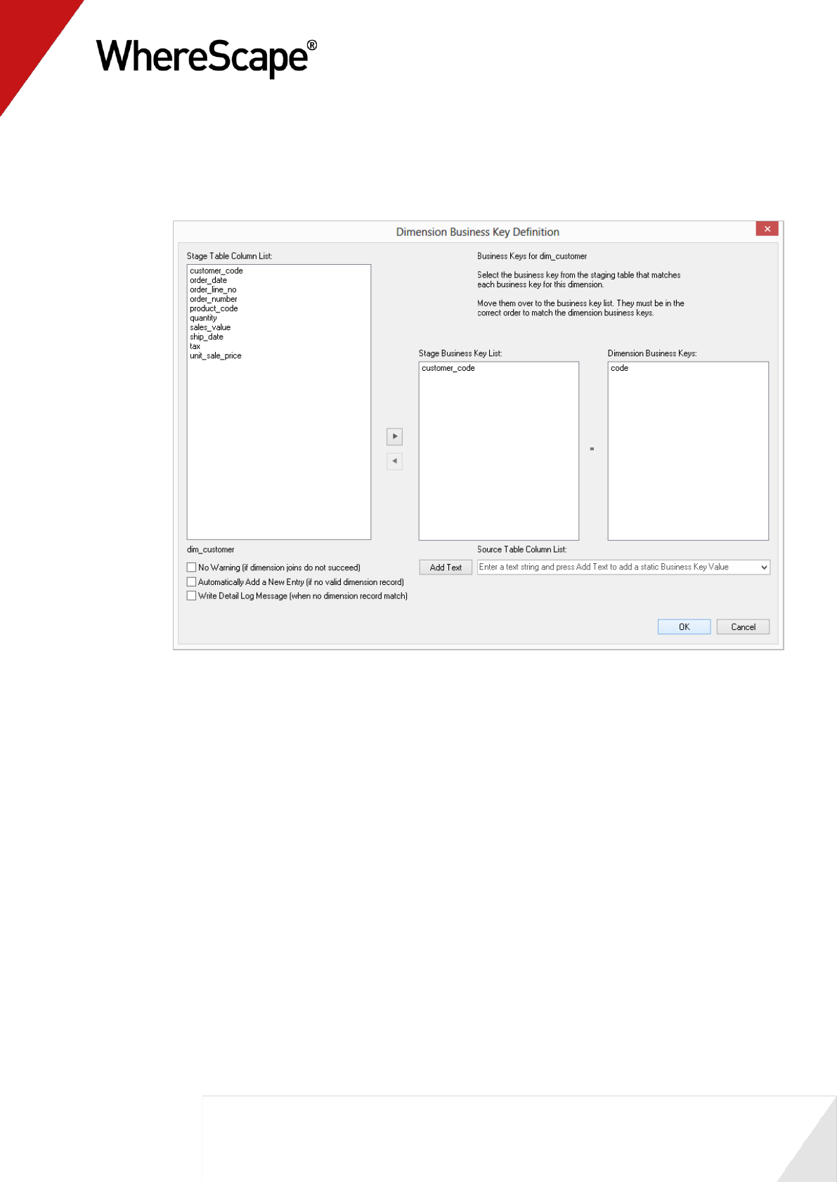
10 You need to match the dimension business keys with the business keys in the stage table.
This associates the correct dimensional record to each stage table record. A dialog box
displays for each dimensional join.
For dim_customer, select customer_code. Click > and OK.
The business key for dim_order_date has the same column name in the stage table and the
dimension view, allowing WhereScape RED to automatically move order_date to the left
side.
For dim_product, select product_code. Click > and OK.
As you progress to dim_ship_date, notice that ship_date has also been automatically
chosen. Click OK again.
56
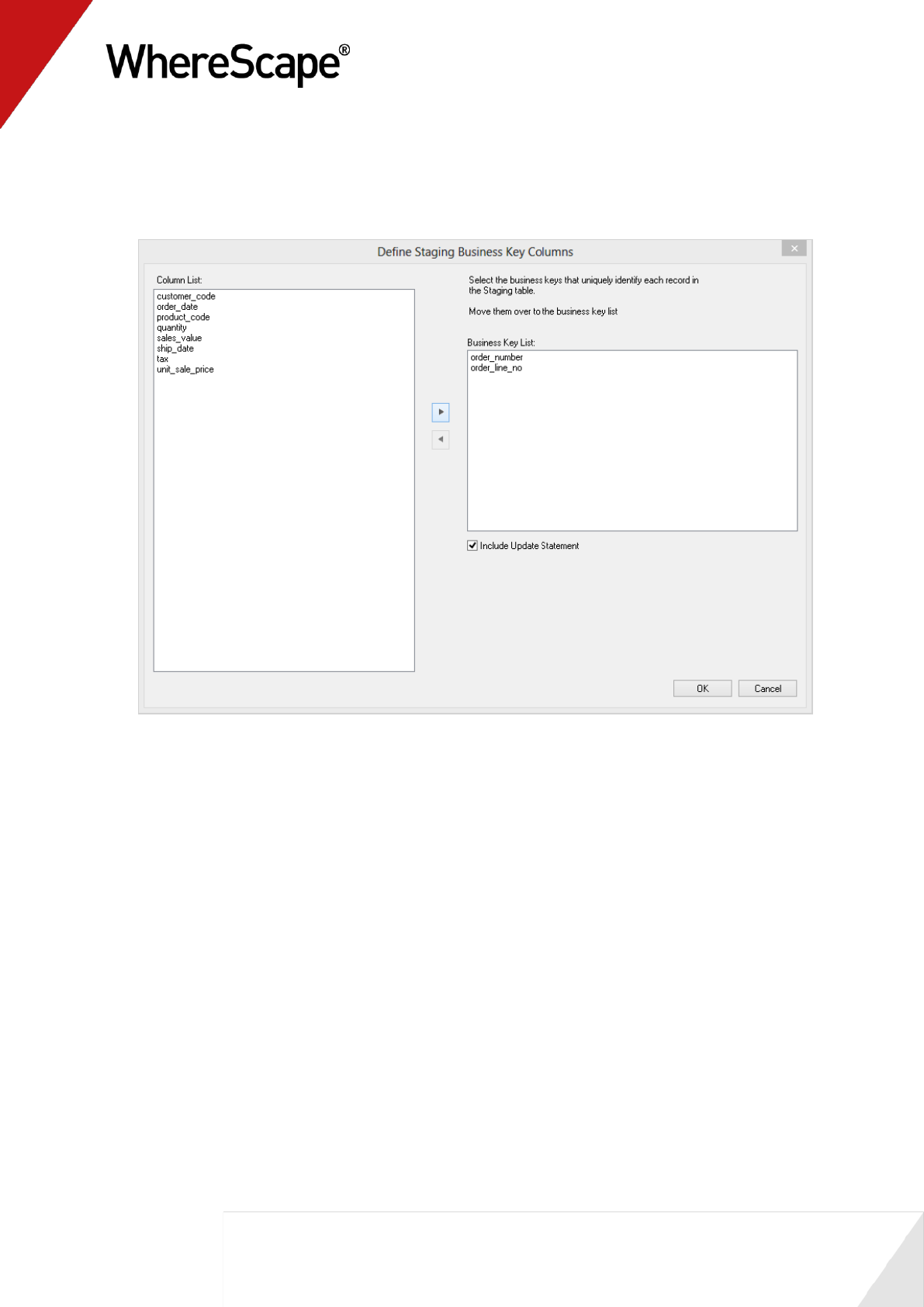
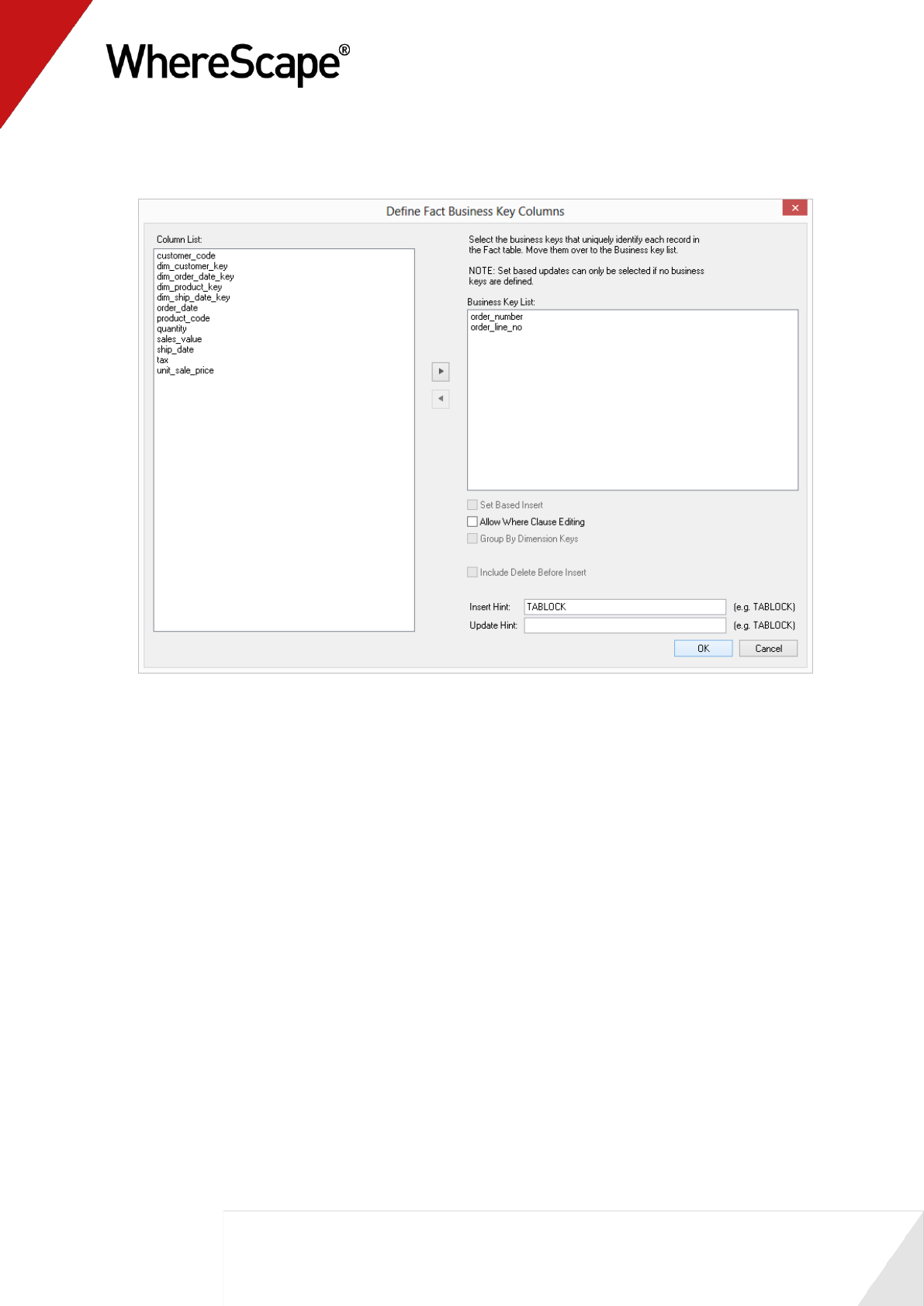
11 Next you must select the business keys to uniquely identify each record in the staging table
itself. This essentially defines the business key we will be using in the fact table, and as such
defines the grain of the fact table. For this example the grain is order line. Select
order_number and order_line_no. Click > and OK.
12 WhereScape RED now builds and compiles the update procedure. The results pane shows any
indexes that were created.
57
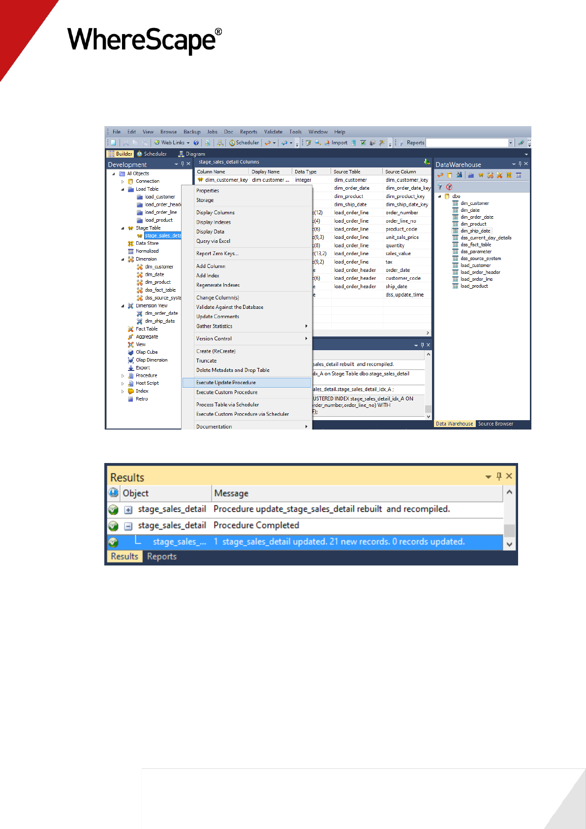
13 The final step is the population of the stage table. Right-click on stage_sales_detail in the
left pane and select Execute Update Procedure.
14 Output from the stage table being updated can now be seen in the Results window.
You are now ready to proceed to the next step - Creating a Fact Table (see "1.12 Creating a Fact
Table" on page 58).
58
1.12 Creating a Fact Table
In this step you will create a fact table.
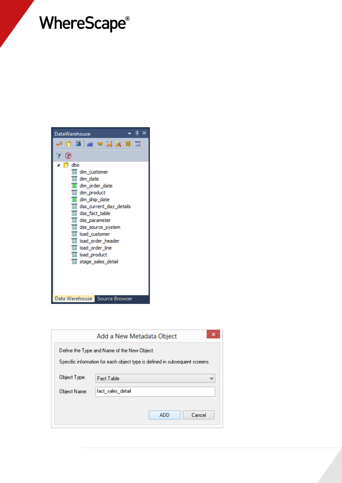
1 Create a drop target by double-clicking on the Fact Table object group in the left pane.
2 Browse the data warehouse connection again (or refresh the data warehouse connection):
3 Drag the stage table stage_sales_detail over from the right pane into the middle pane. The
following dialog is displayed. Click ADD.
59
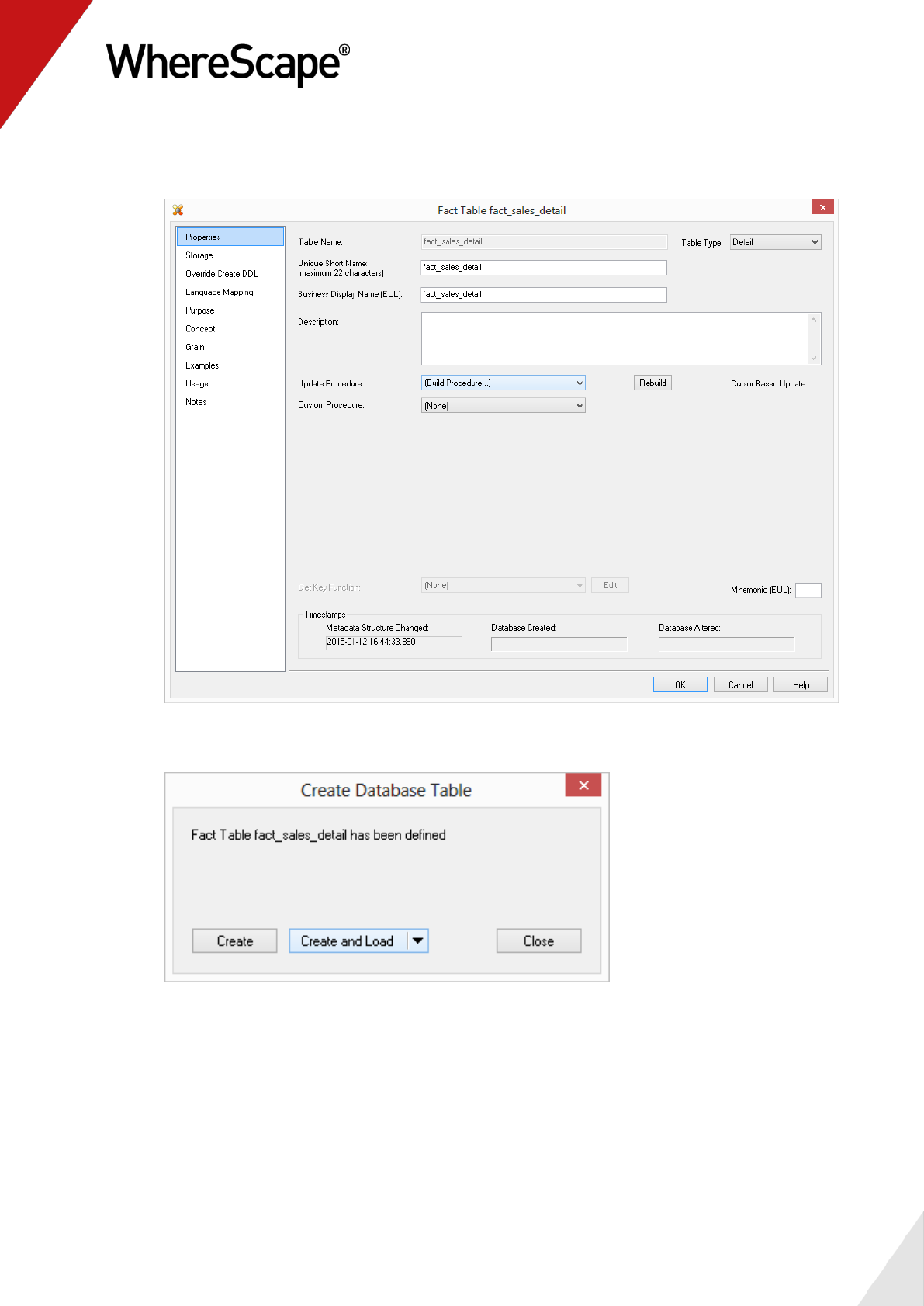
4 The fact_sales_detail table Properties dialog will appear. Select (Build Procedure...) in the
update procedure drop-down and click OK.
5 Select Create and Load to create and load the table now.
60
6 Select the Business Key for the fact table. Choose order_number and order_line_number.
Click > and then OK.
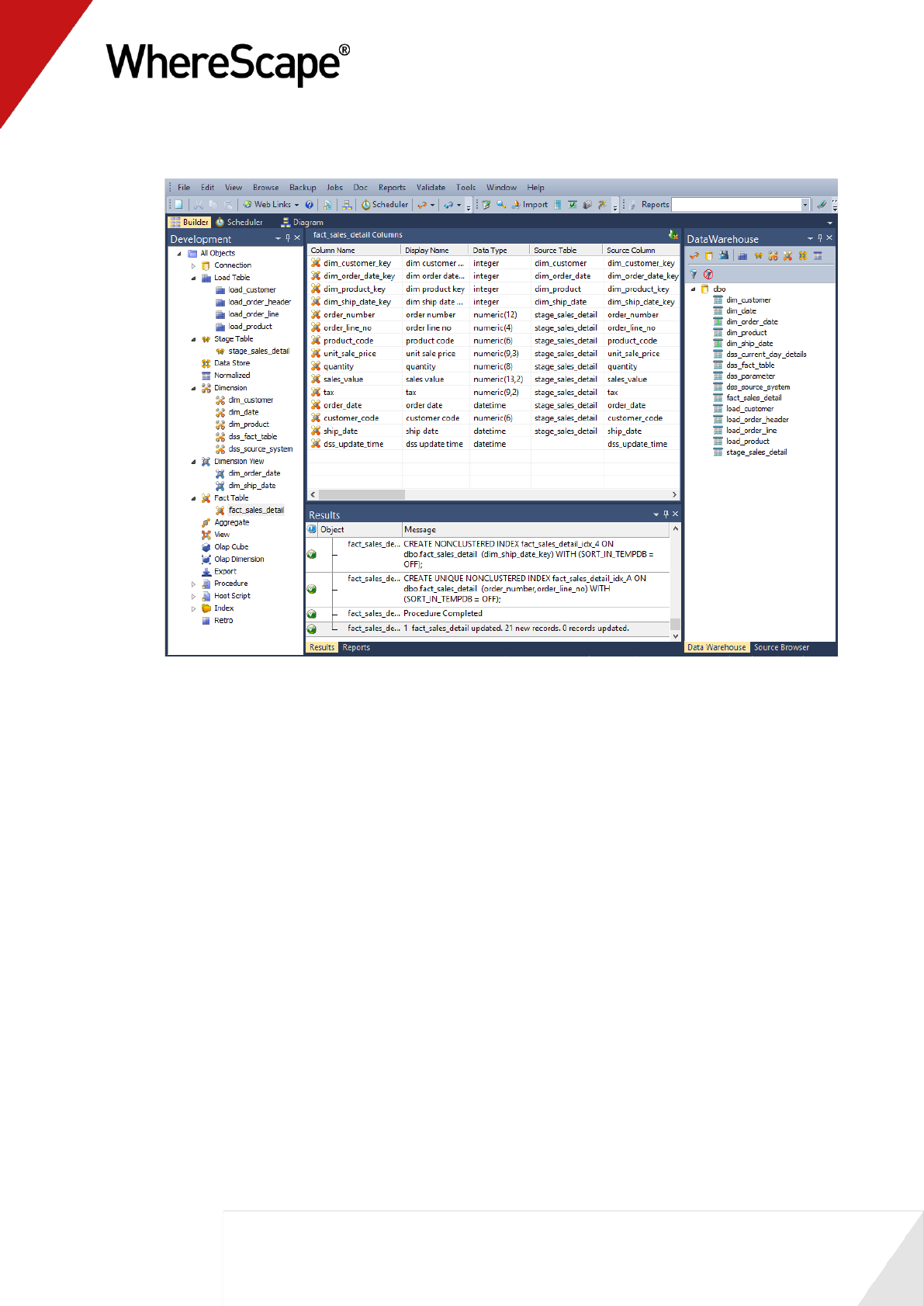
7 Output from the fact table being created and updated can now be seen in the Results window.
Refresh the Data Warehouse in the right pane.
62
1.13 Switching to Diagrammatic View
WhereScape RED provides the ability to diagrammatically view the data warehouse you have
created.
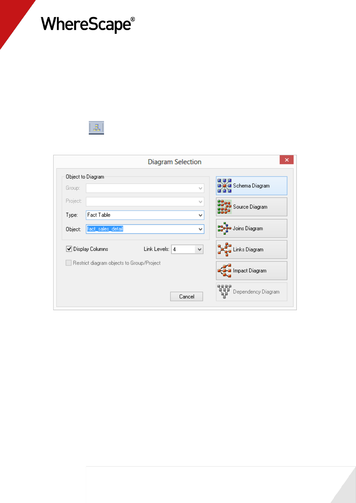
1 Click on the button to display the Diagram Selection dialog.
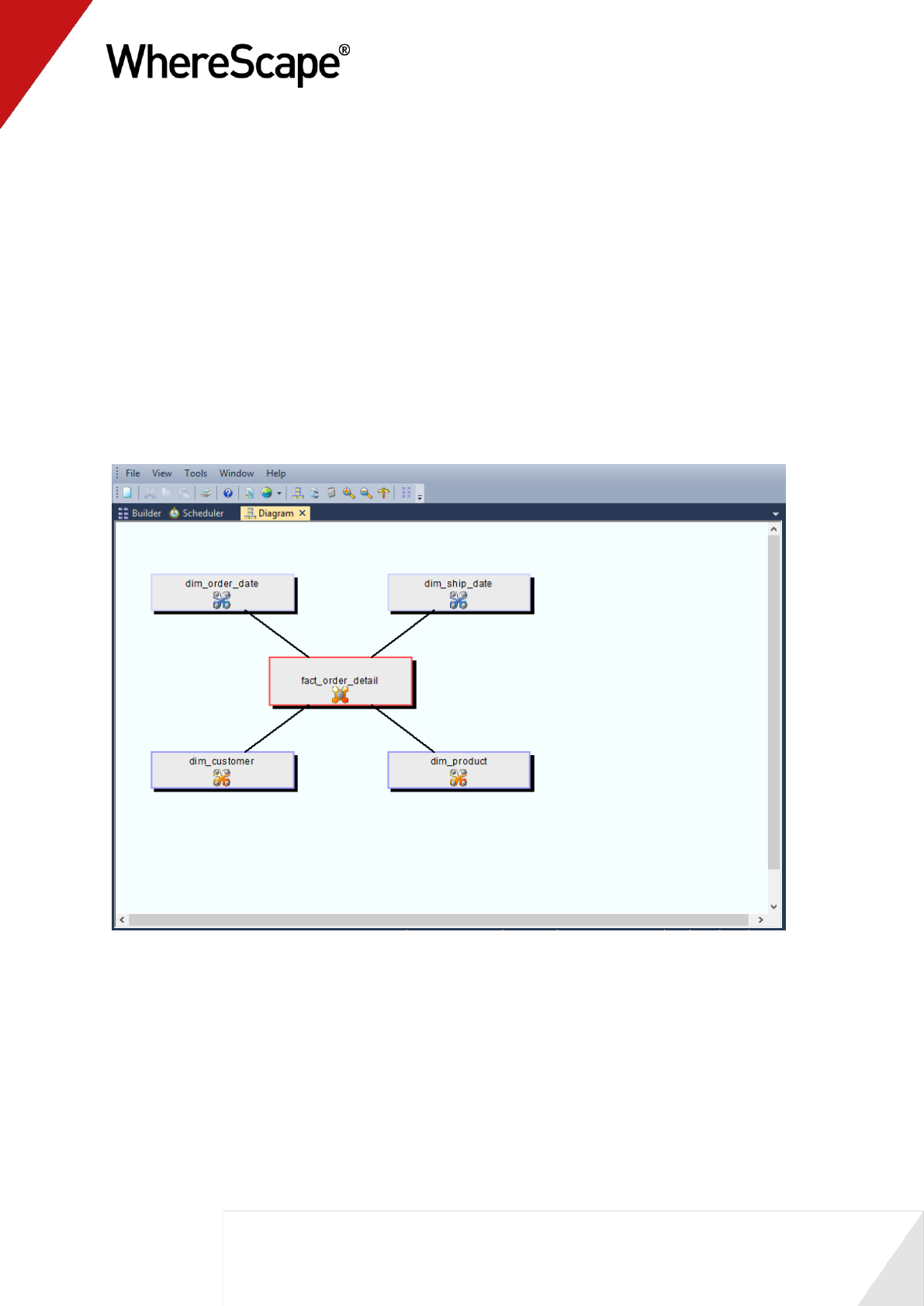
2 Select an object Type of Fact Table to narrow the selection list and then select
fact_sales_detail. Click on the Schema Diagram button to display a star schema diagram.
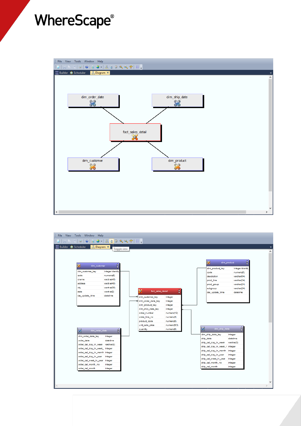
63
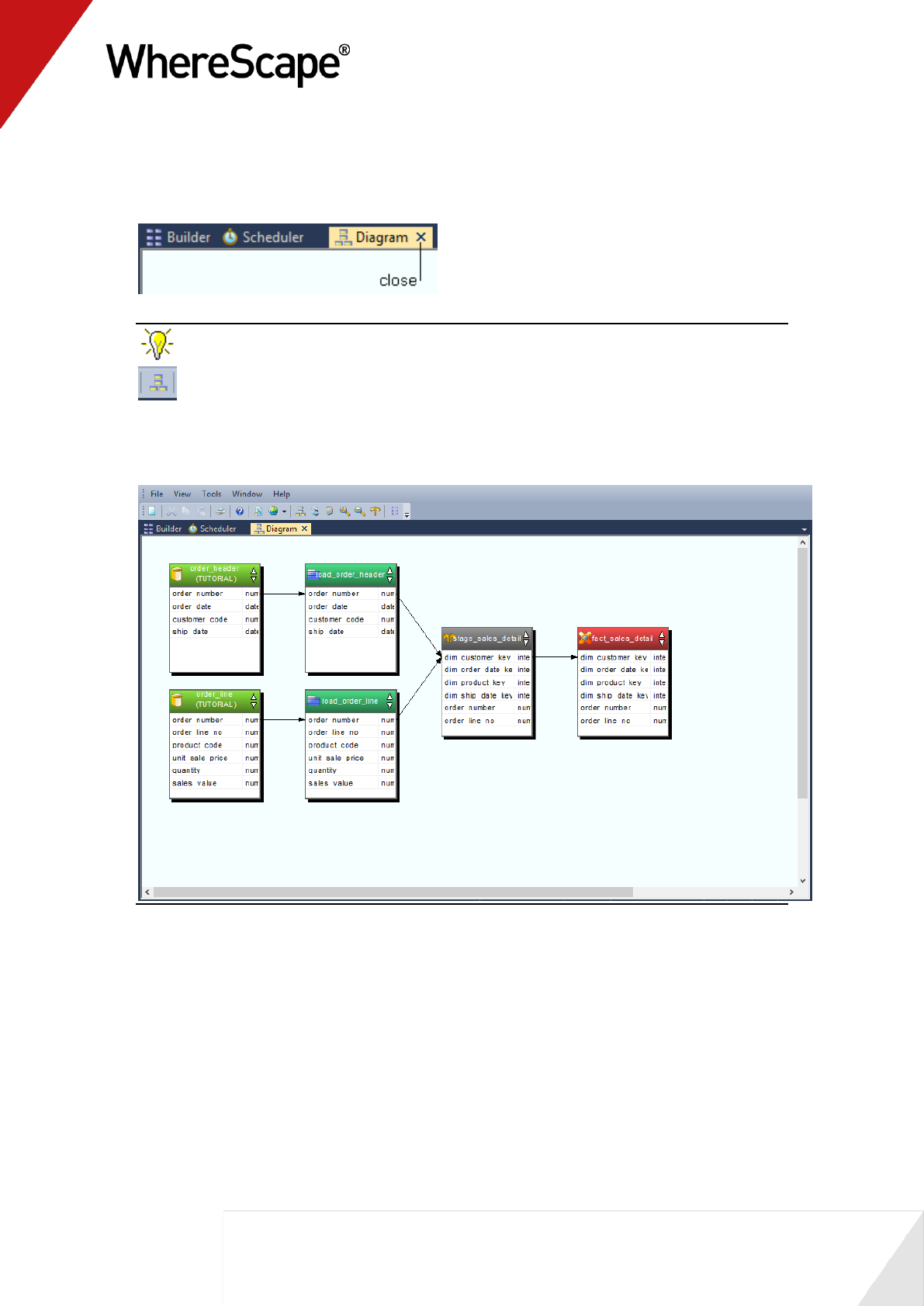
The diagram looks like this:
The toggle button will enable you to switch between the detailed and standard diagrams.
64
3 To close the diagrammatic view, click on the X on the diagram tab, or alternatively, return to
the Builder section by clicking the Builder tab.
TIP: To view the source tracking of the fact_sales_detail table, click once more on the
button, choose the fact_sales_detail table and then click on the Source Diagram
button.
The diagram looks like this:
You are now ready to proceed to the next step - Producing Documentation (see "1.14
Producing Documentation" on page 65).
65
1.14 Producing Documentation
WhereScape RED also provides the ability to produce user and technical documentation.
This is obviously of more value if the descriptive data has been entered against the columns and
tables in the data warehouse, which we have not done during this tutorial.
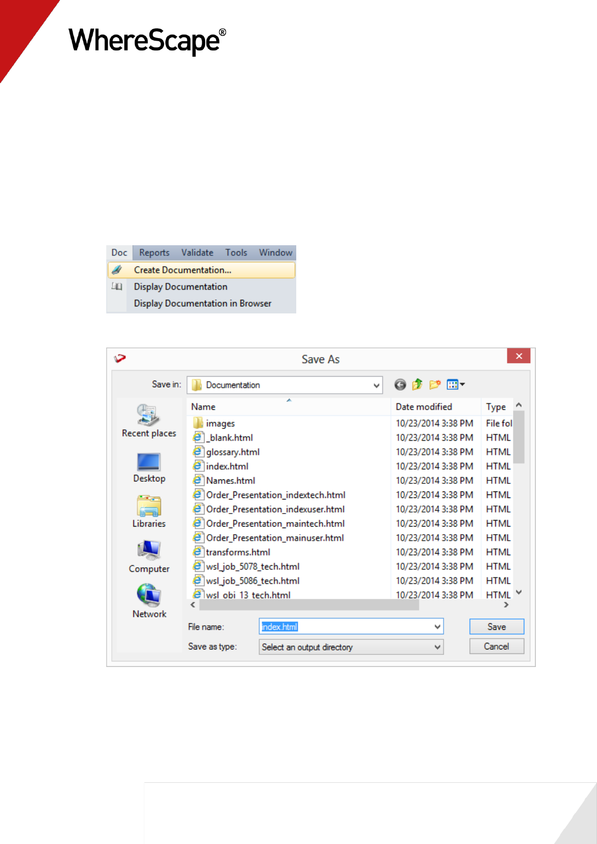
1 To view the documentation for the components of the data warehouse, select Doc from the
menu, then Create Documentation.
2 Select a file path (directory) under which to save the HTML files that will be produced.
66
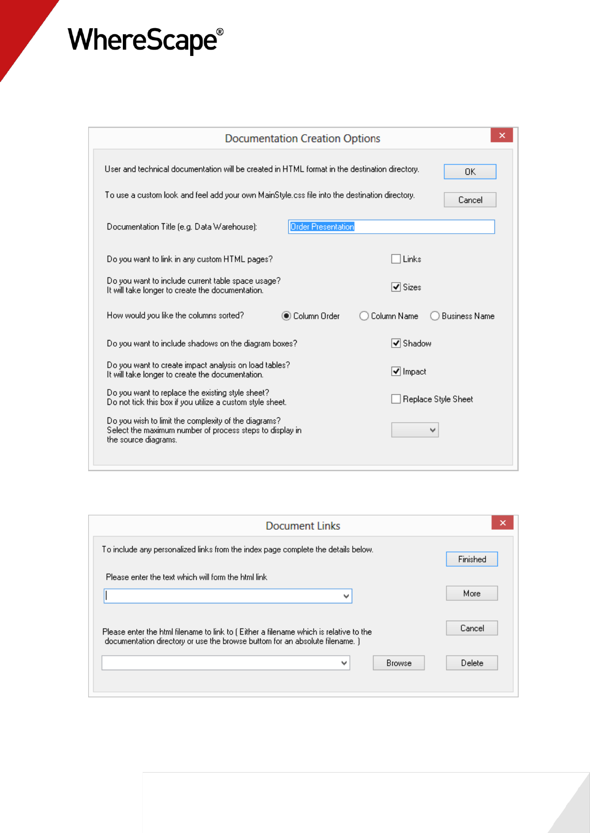
3 The next screen allows for the inclusion of a banner and user defined links. Leave these
options unchecked and click OK to proceed.
4 Include any personalized links if required and click Finish.
68
1.15 Data Store Objects (Optional)
Data Store objects are used to provide a persistent storage of load tables. These objects are not
licensed for every installation and hence this section is optional.
1 Browse the Data Warehouse in the right pane.
2 Double-click the data store object in the left pane.
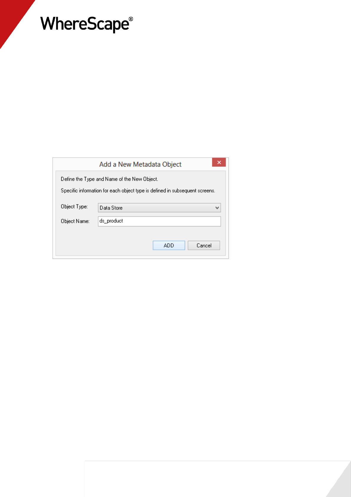
3 Drag load_product from the right pane into the middle pane.
4 Accept the default name of ds_product and click ADD.
69
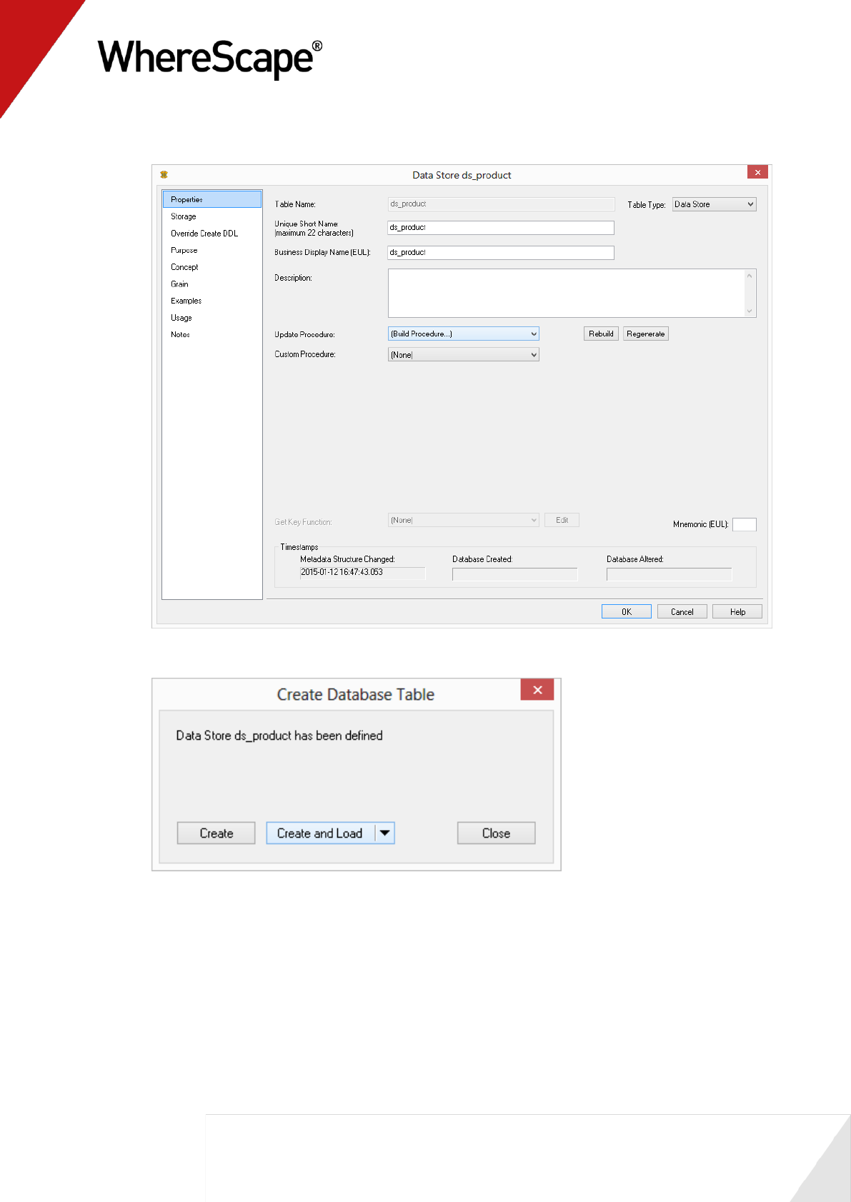
5 Select (Build Procedure...) from the Update Procedure drop-down list. Click OK.
6 Click Create and Load.
70
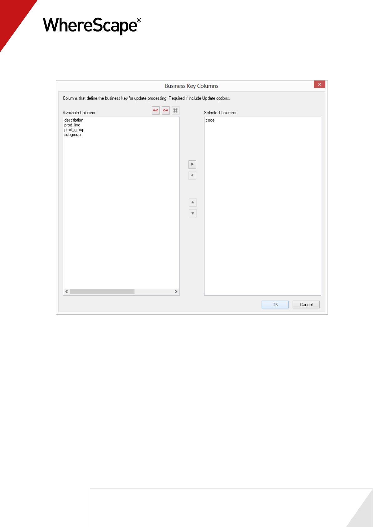
7 Select code as the business key by clicking on the ellipsis button to the right of the Business
Key Columns field by clicking code, selecting > or by double-clicking on code. Click OK.
71
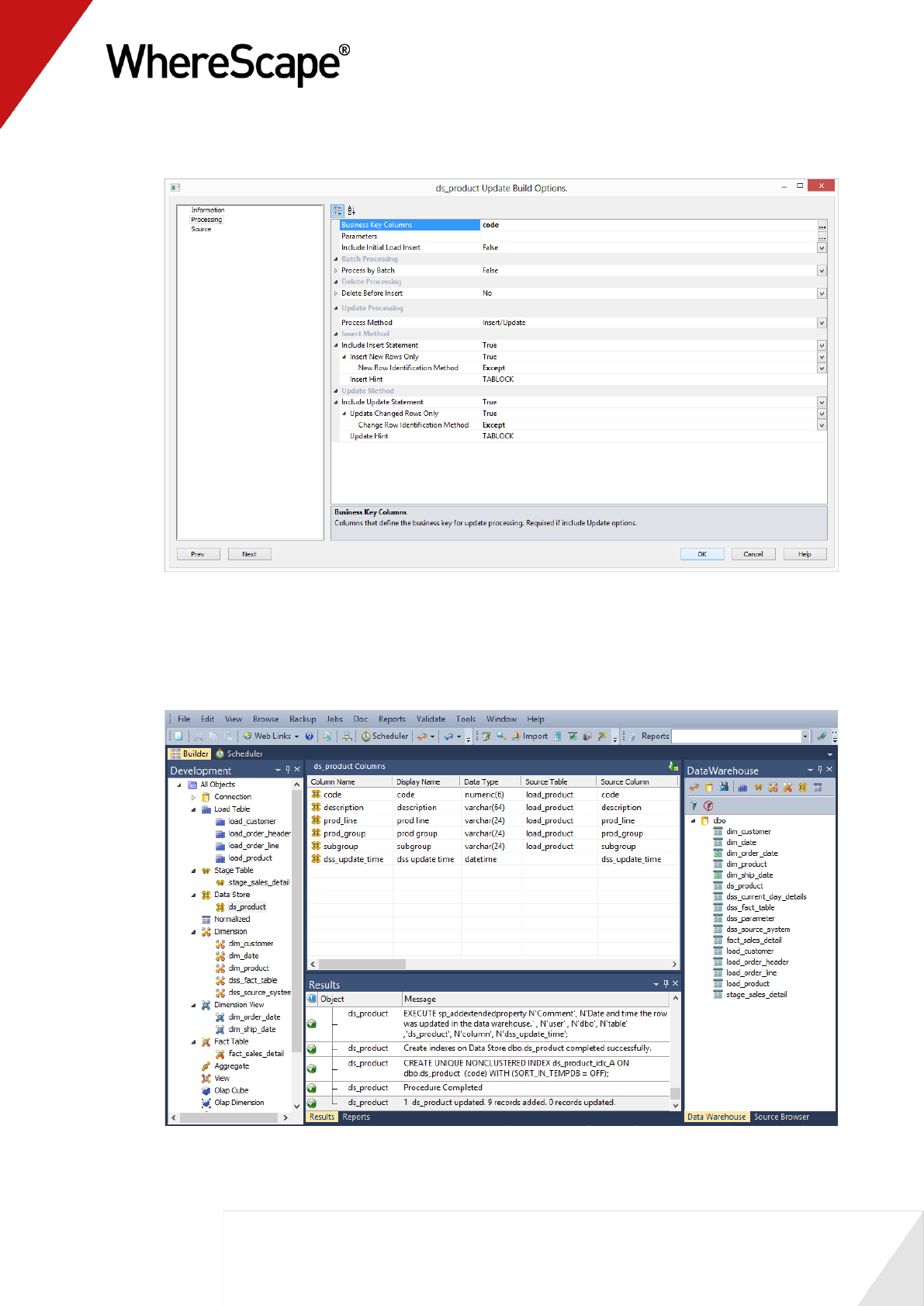
8 Make sure the options as set as shown below and click OK.
9 Data should now be loaded into the ds_product table. Refresh the Data Warehouse in the right
pane (F5).
10 Your screen should look something like this:

72
11 Repeat the exercise for order_line, order_header and customer.

73
Before you start on this chapter you should have:
Completed Tutorial 1 - Basic Star Schema Fact Table (see "Basic Star Schema Fact Table"
on page 1)
Successfully completed Creating a Fact Table (see "1.12 Creating a Fact Table" on page 58)
This chapter deals with fine tuning the data warehouse by creating roll-up fact tables and
aggregates. It also includes loading an ascii file into a new load table.
In This Tutorial
2.1 Purpose and Roadmap.................................................. 74
2.2 Creating a Connection to Windows ............................. 77
2.3 Loading Tables from Flat Files ..................................... 81
2.4 Creating Stage Tables................................................... 87
2.5 Creating Fact Tables..................................................... 89
2.6 Rollup/Combined Fact Table ........................................ 91
2.7 Aggregate Tables .......................................................... 95
2.8 Creating a Customer Aggregate ................................... 98
T u t o r i a l 2
Rollup Fact Tables, ASCII File Loads,
Aggregates
74
2.1 Purpose and Roadmap
Purpose
This tutorial will walk you through the process to:
Load data from flat files (in Tutorial 1 source data was obtained via database links)
Create a rollup fact table that allows users to see budgeted, forecast, and actual sales
amounts and quantities broken down by customer, product and month
Create separate aggregate tables that summarize data in the rollup table by (i) product and
(ii) customer
In short, this tutorial loads budget and forecast data from flat files into their own load, stage and
fact tables. This data is then combined with data from the fact_sales_detail table (created in
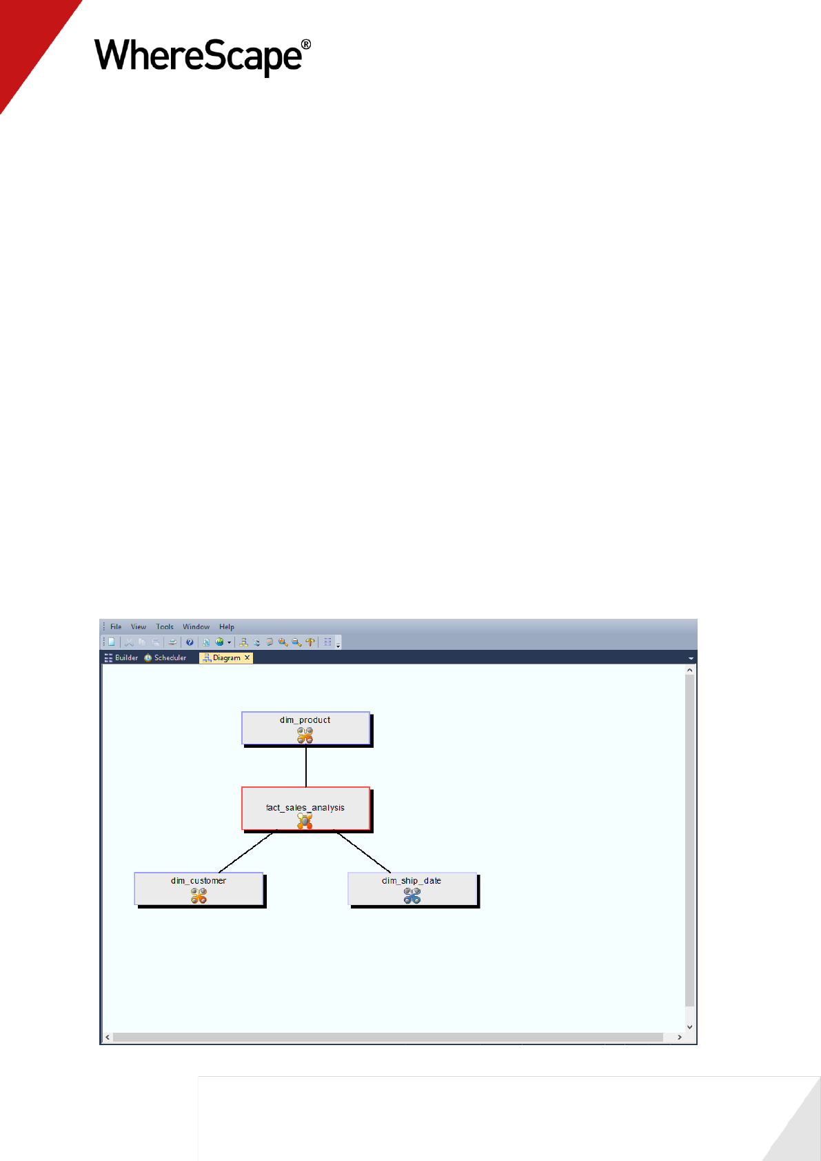
Tutorial 1) and summarized to create a new rollup fact table, fact_sales_analysis. Further
summarization is done on the rollup table to create two separate aggregate tables.
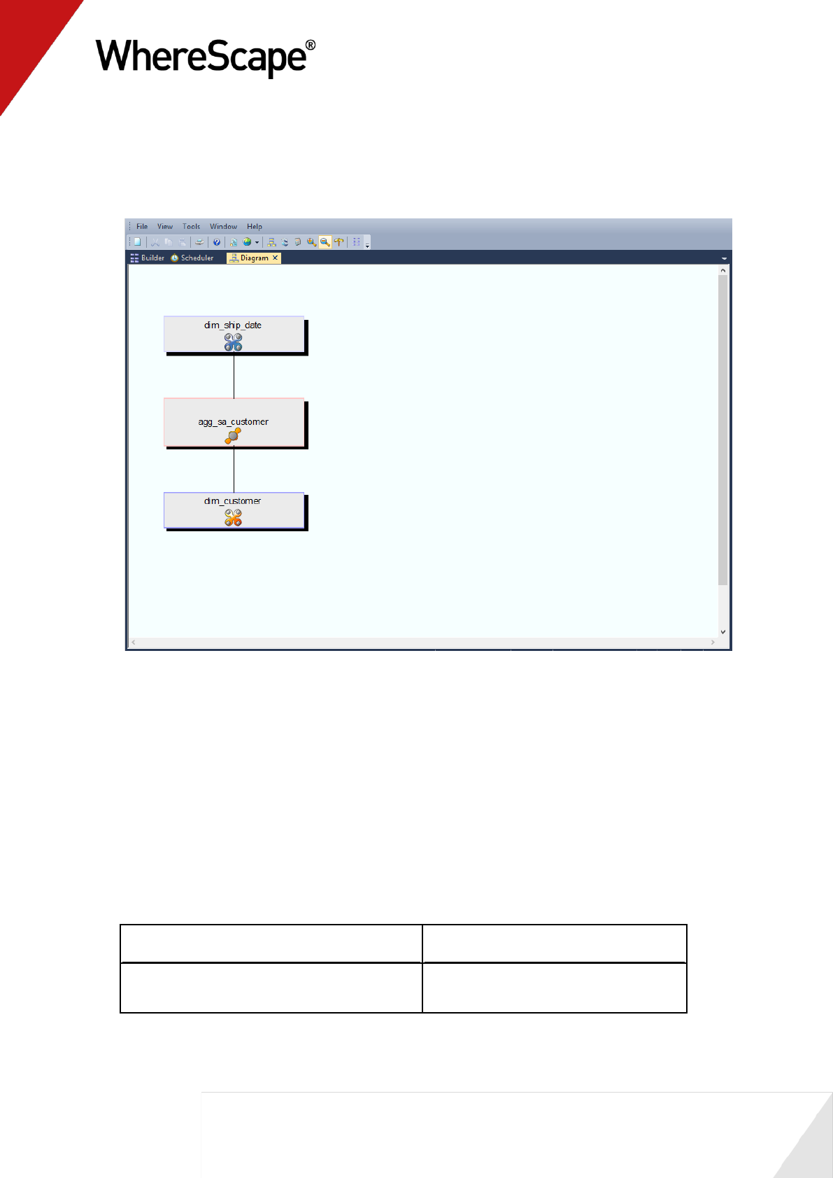
The following are diagrams showing (i) the rollup table, fact_sales_analysis and (ii) the customer
aggregate table, agg_sa_customer that will be created as part of this tutorial.
Rollup fact_sales_analysis:
75
Aggregate agg_sa_customer:
Tutorial Environment
This tutorial has been completed using IBM DB2. All of the features illustrated in this tutorial are
available in SQL Server, Oracle and DB2 (unless otherwise stated).
Any differences in usage of WhereScape RED between these databases are highlighted.
Tutorial Roadmap
This tutorial works through a number of steps. These steps and the relevant section within the
chapter are summarized below to assist in guiding you through the tutorial.
Step in Tutorial
Section
Create a new connection to allow data to be
loaded in from flat files on C: drive.
Making a Connection to Windows
76
Step in Tutorial
Section
Create (and load) the data for
load_budget
load_forecast
Note: Data is loaded from flat files on C: drive
Loading Tables from Flat Files
Create the following stage tables
stage_budget
stage_forecast
Stage table creation entails using
corresponding load tables and including links
to the following dimensions: (dim_customer,
dim_product, dim_date)
Creating Stage Tables
Create the following fact tables
fact_budget
fact_forecast
Creating Fact Tables
Create the rollup fact table, fact_sales_analysis
This rollup combines forecast, budget and
sales data from fact_budget, fact_forecast and
fact_sales_detail tables respectively. The data
is rolled-up (grouped) by product, customer
and month. Note that dimension keys are used
for the rollup.
Rollup/Snapshot Fact Tables
Create product aggregate (agg_sa_product)
table.
This aggregate summarizes fact_sales_analysis
data by product
Aggregate Tables
Create customer aggregate (agg_sa_customer)
table.
This aggregate summarizes fact_sales_analysis
data by customer.
Creating a Customer Aggregate
This tutorial starts with the section Making a Connection to Windows (see "2.2 Creating a
Connection to Windows" on page 77).
77
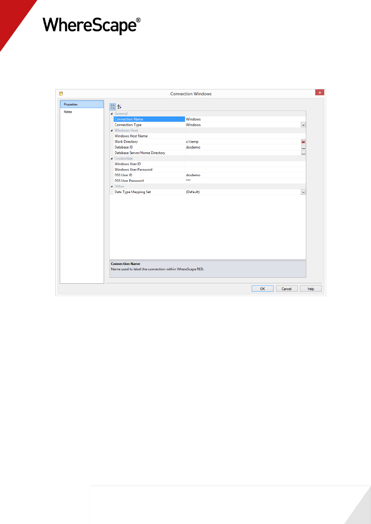
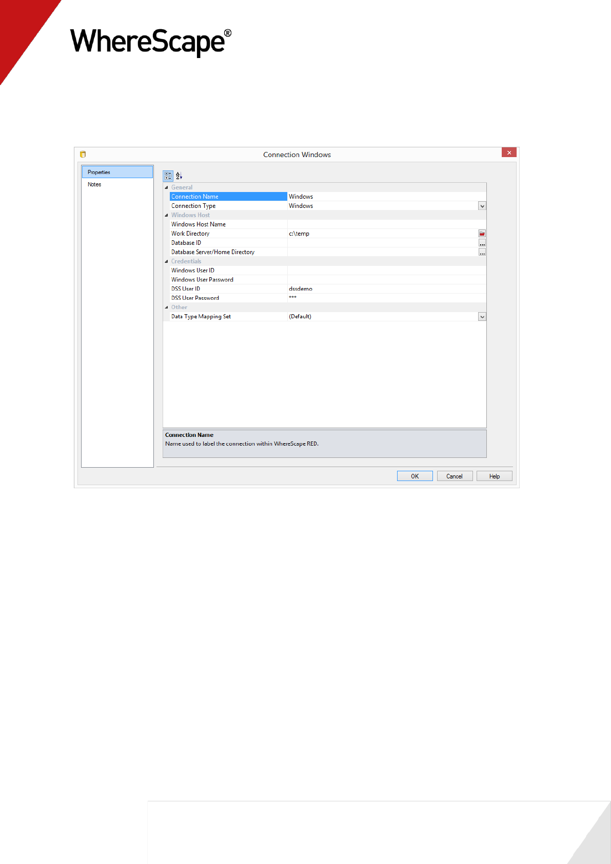
2.2 Creating a Connection to Windows
This follows a similar process to the earlier connections (see "1.6 Creating a Connection" on page
14) made, but differs in that the connection is within the computer.
Note: The following connection should have been automatically created. It should however be
validated to ensure that it is correct for the environment.
1 Log on to WhereScape RED.
2 In the left pane, double-click on the Connection object group.
3 Select File | New, or right-click the Connection object and select New Object.
4 Enter Windows in the 'Name of Object' text box and select Add.
5 Enter the Connection properties as below:
Field
Description
Connection Name
Windows
Connection Type
Windows
Host Name
Not required
Work Directory
Required. Must be an existing valid directory on the PC, e.g,
c:\temp
Database id (SID)
For Oracle, the appropriate SID for your metadata
installation, e.g. ORCL. For SQL Server and DB2 leave this
field blank.
Database home
directory
This is only required for Oracle and if the Database SID is in a
non-default directory
Windows User ID
Leave blank
Windows Password
Leave blank
Dss User ID
For Oracle, this is the data warehouse username. This is the
database logon for SQL Server and DB2. It should be dbo if a
trusted connection is being used for SQL Server. If an OS
authenticated user is being used for DB2 this should be left
blank.
Dss password
For Oracle, this is the data warehouse password. This is the
database password for SQL Server and DB2. It should be left
blank if a trusted connection is being used for SQL Server or if
an OS authenticated user is being used for DB2.

78
Sample SQL Server Properties
79
Sample Oracle Properties:
81
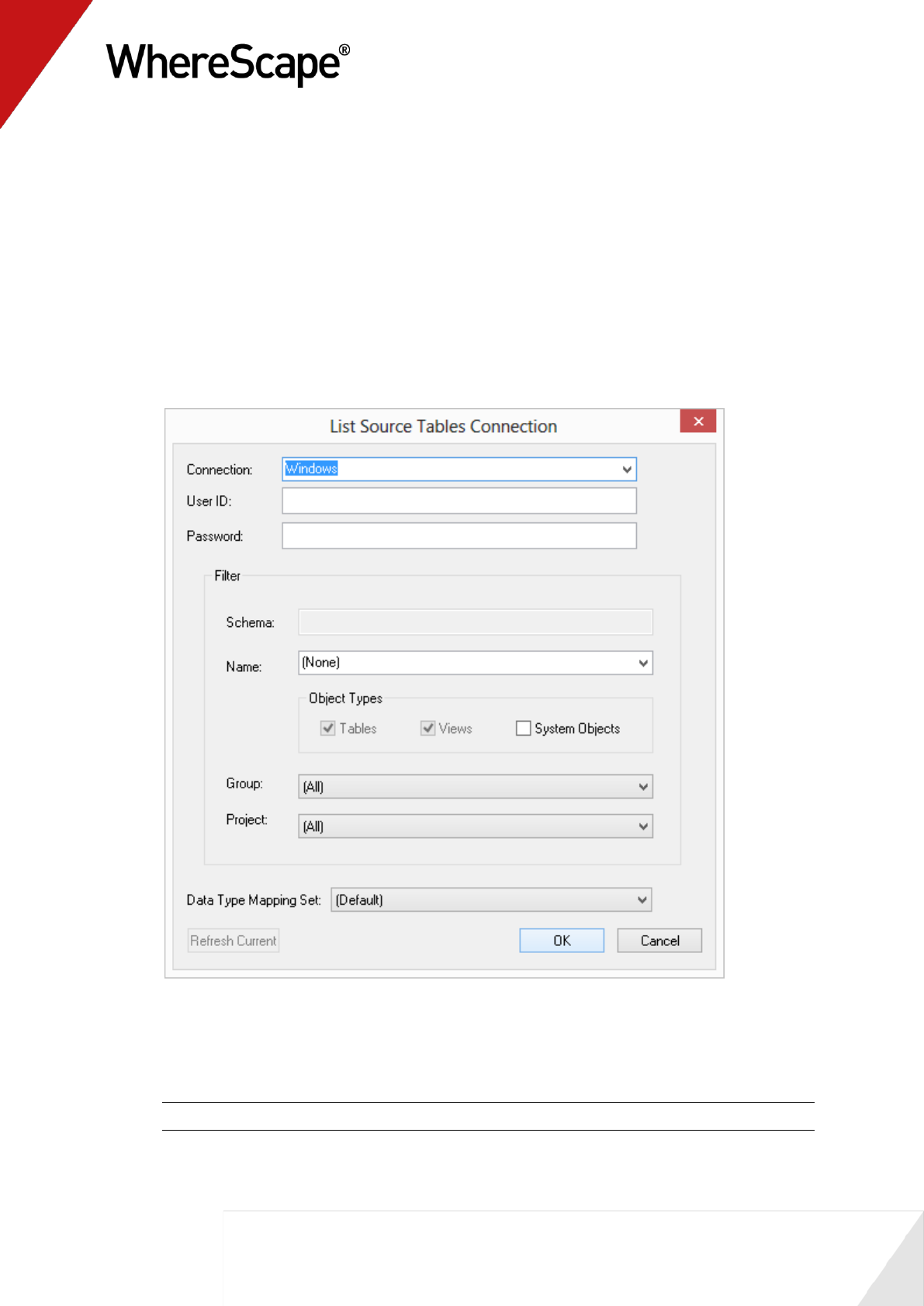
2.3 Loading Tables from Flat Files
In this step you will parse and load a file from Windows into a load table in the data warehouse.
1 Double-click on the Load Table object group in the left pane. This will list all load tables in
the middle pane and make the middle pane a drop target for new load tables.
2 Browse to the Windows connection in the right pane by selecting Browse | Source Tables
from the menu strip at the top of the screen.
3 Select Windows as the Connection. Leave the Schema field blank. Click OK.
4 In 32 bit systems navigate to c:\Program Files\WhereScape\Tutorial folder, click on
budget.txt and drag it into the middle pane.
5 For 64 bit systems, navigate to c:\Program Files (x86)\WhereScape\Tutorial instead.
The path above may be different if WhereScape has not been installed in the default location.
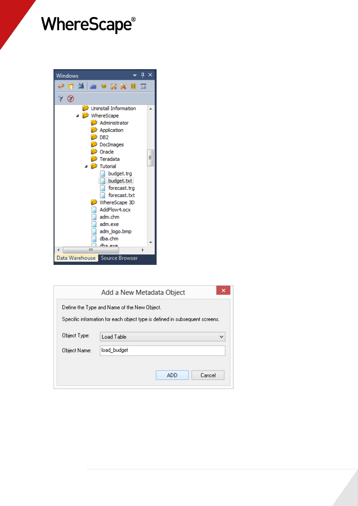
82
6 Accept load_budget as the object name and click ADD.
83
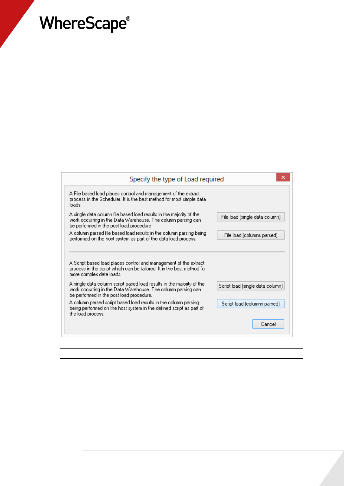
Specifying the load type
You must now specify the type of load you require from the four options given:
File load (single data column)
File load (columns parsed)
Script load (single data column)
Script load (columns parsed)
For more information on load types see the section on flat file loads in the loading data chapter.
1 For this tutorial select Script load (columns parsed).
Note: For DB2, file loads are not available in this dialog.
84
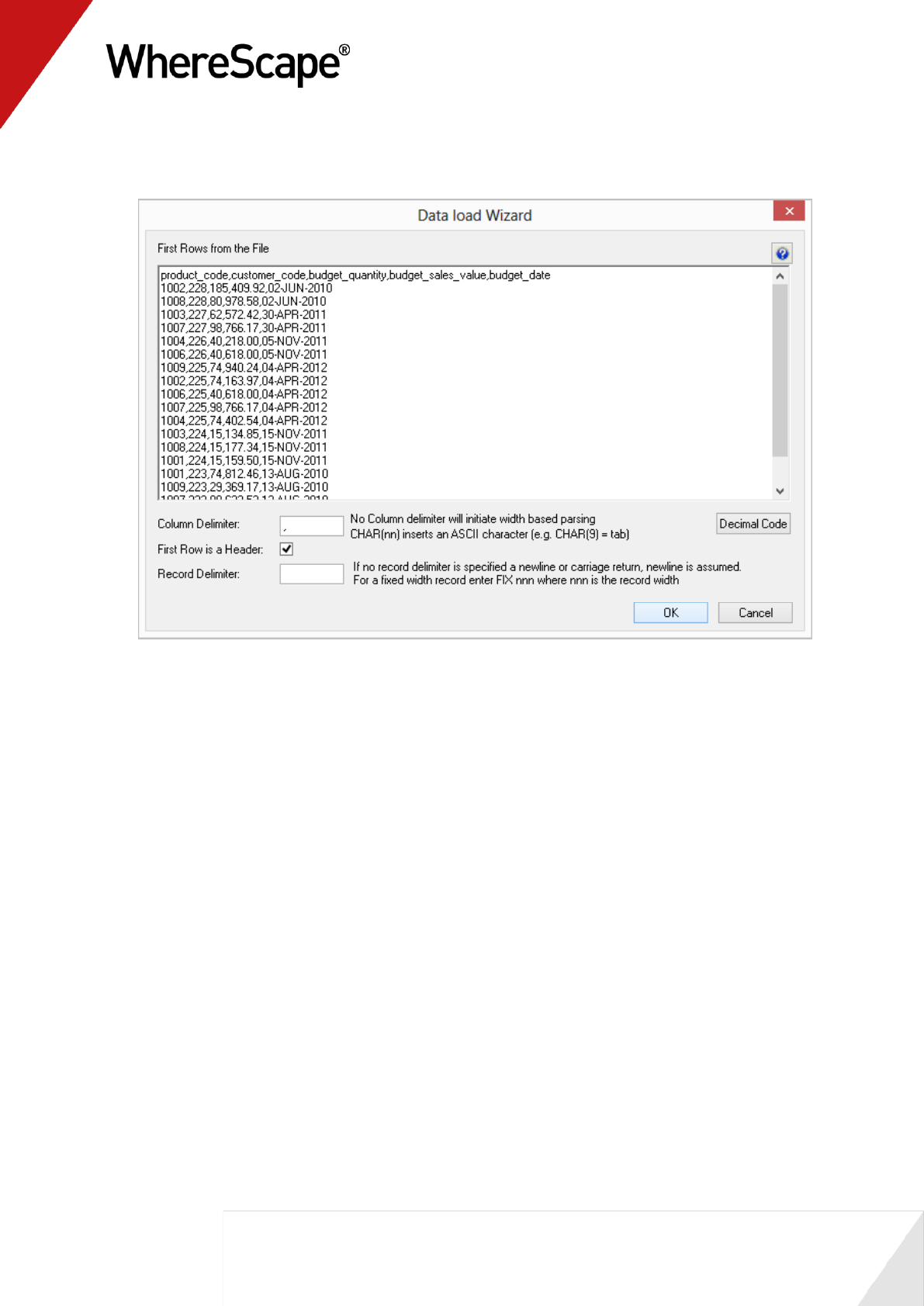
2 From the data load wizard enter a comma (,) in the Column Delimiter field. As the first row is
a header, place a check in the box and click OK.
85
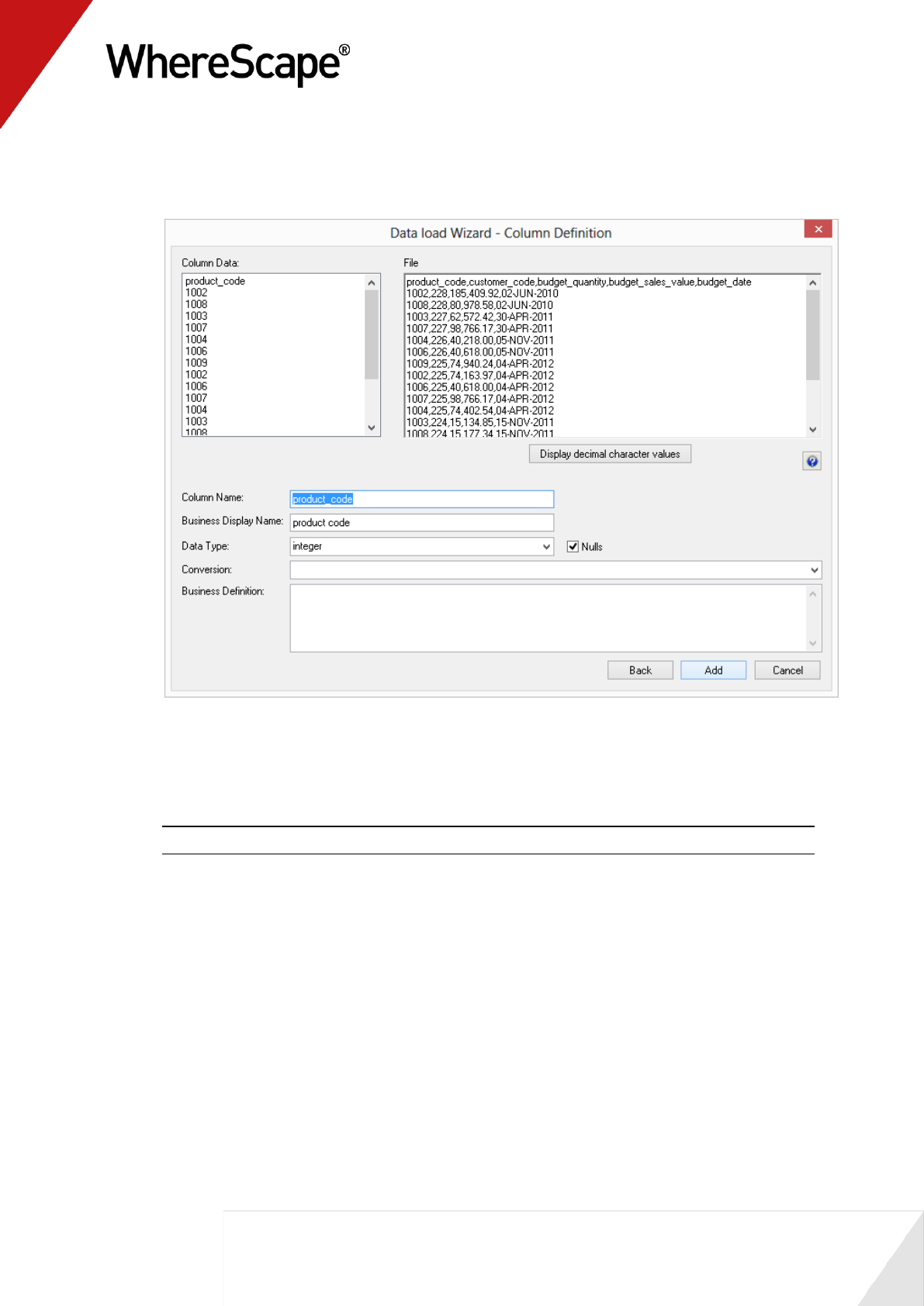
3 WhereScape RED uses the header row as suggested column names. For each following column
confirm the name and data type. You may have to change it to a more appropriate value.
Click Add.
4 Click OK on the load_budget Properties dialog.
5 Click OK for the DB2 Load cannot skip header rows dialog.
6 Click OK on the New script created dialog.
7 Select Yes on the prompt to create and load the table now.
Note: Loading files with a header row into DB2 will result in an error message.
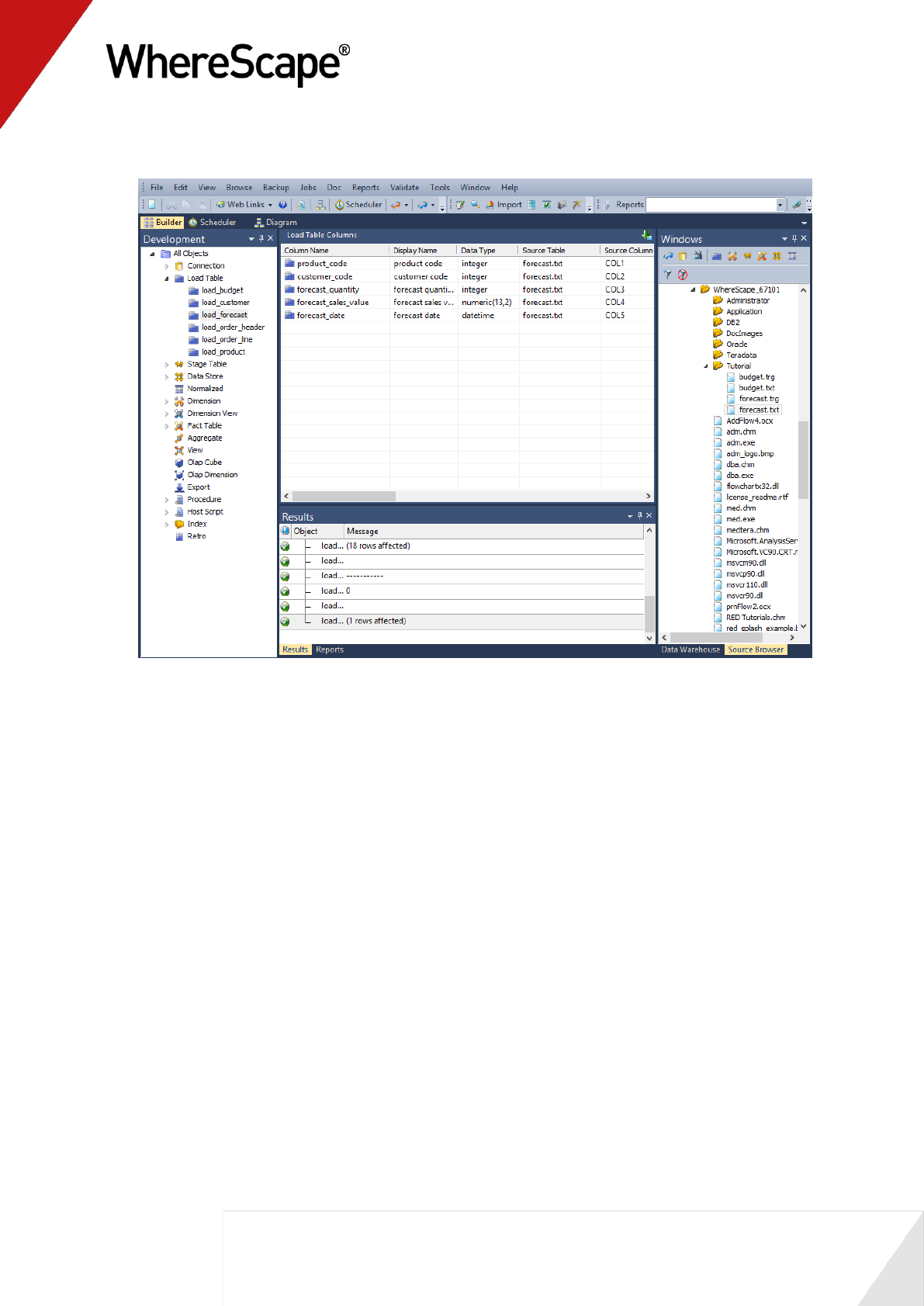
8 Repeat steps (1) to (9) for the forecast.txt file to create and load the table load_forecast.

87
2.4 Creating Stage Tables
Two separate stage tables need to be created for load_budget and load_forecast. This is the
same as the procedure from the first tutorial for Defining the Staging Table (see "1.10 Defining
the Staging Table" on page 45).
1 Double-click the stage table object group in the left pane. This will list the existing stage
table in the middle pane.
2 Browse to the data warehouse Browse/Source Tables or click on the orange glasses in the
toolbar.
3 Drag the table load_budget from the right pane to the middle pane and drop.
4 Click ADD to add the stage table called stage_budget.
5 Click OK on the Properties dialog.
6 Now bring in the following keys from the right pane into the new table. Click the stage table
name in the left pane to list the stage table columns in the middle pane; this also makes the
middle pane a drop target for new columns:
- dim_customer_key
- dim_product_key
- dim_date_key
7 Now in the left pane, right-click on stage_budget and select Create (ReCreate).
8 In the left pane, right-click on stage_budget and select Properties. In the Update Procedure
field select (Build Procedure...). Click OK.
9 Select Cursor as the update procedure type.
10 Click OK on the Parameters dialog.
11 SQL Server data warehouse users will now see an additional join screen. This screen is
presented even though no joins are required. This screen allows the selection of either a
'Where' based join or an ANSI standard join. The default will be ANSI standard join. Click OK
to proceed.
12 Select the dimension keys:
dim_customer - customer code
dim_product - product code
dim_date - budget/forecast date (depending on which stage table you are working on).
Click > then OK for each one.
13 Now define the business keys. Add customer_code, product_code, and
budget/forecast_date to the business key list, and click OK.
14 Right-click on the stage table in the left pane, and select Execute Update Procedure.
15 Repeat steps (1) to (14) to create stage table stage_forecast from load_forecast.
16 Refresh the Data Warehouse in the right pane (F5).

89
2.5 Creating Fact Tables
1 Double-click on the Fact Table object group in the left pane.
2 Click and drag stage_budget into the middle pane. Accept the name fact_budget and click
ADD.
3 Select (Build Procedure...) from the update procedure drop-down list and click OK.
4 Click Create and Load when asked if you wish to create and load the table now.
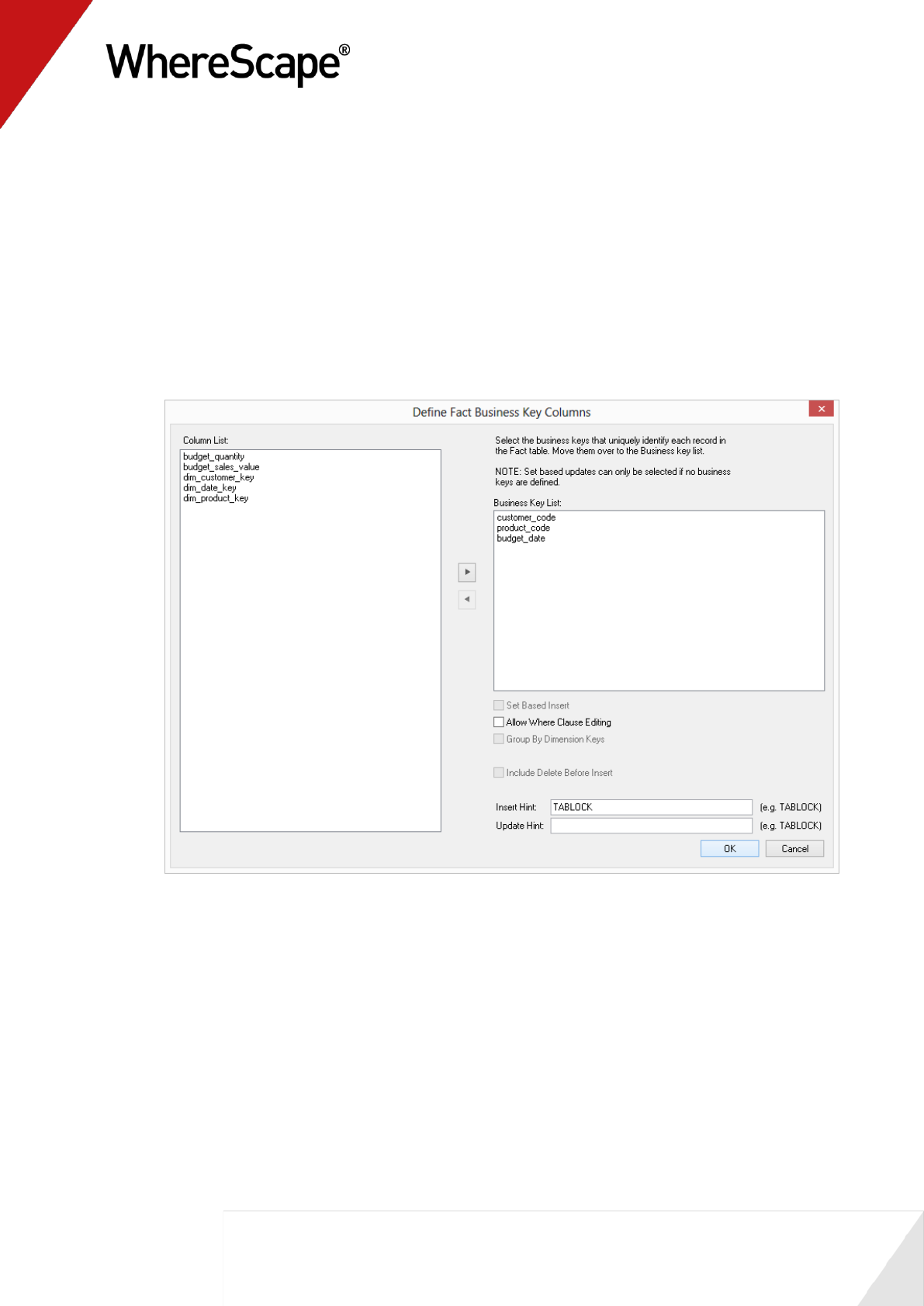
5 Select the Business Key definitions. Add customer_code, product_code, and budget_date
and click OK.
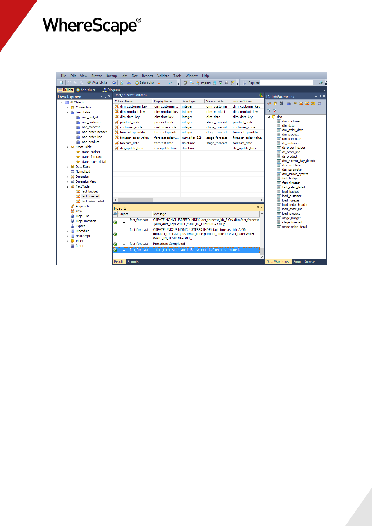
6 Repeat steps (1) to (5) on stage_forecast to create fact_forecast (with a business key of
customer_code, product_code, and forecast_date).
7 Refresh the Data Warehouse in the right pane (F5).

91
2.6 Rollup/Combined Fact Table
A rollup table enables the viewing and combining of different levels of granularity in the data,
such as sales, budget and forecast detail. The result is that the end user can compare, for
example, sales against budget against forecast on a monthly basis.
1 Double-click on the Fact Table object group in the left pane.
2 Click and drag fact_sales_detail to the middle pane, and change the new object name to
fact_sales_analysis.
Note: Do not make any changes to the table definition and click Close when asked if you
want to create and load the table now.
3 Because this level of granularity is no longer required, delete the following columns:
customer_code
product_code
order_date
ship_date
dim_order_date_key
unit_sale_price
order_number
order_line_no
Note: A new column has appeared - dss_fact_table_key. This is used to identify which fact
table has populated a row in the rollup fact table and should not be removed.The
dss_update_time field must also be present to record the time that the record was updated in
the data warehouse
92
4 In the left pane click the fact_sales_analysis table. In the right pane open fact_budget and
drag budget_quantity and budget_sales_value into the middle pane (within
fact_sales_analysis).
5 In the right pane open fact_forecast and drag forecast_quantity and forecast_sales_value
into the middle pane (within fact_sales_analysis).
6 In the left pane, right-click on fact_sales_analysis and select Create (ReCreate).
7 In the left pane, again right-click on fact_sales_analysis and select Properties. In the Update
Procedure field select (Build Procedure...) and then click OK.
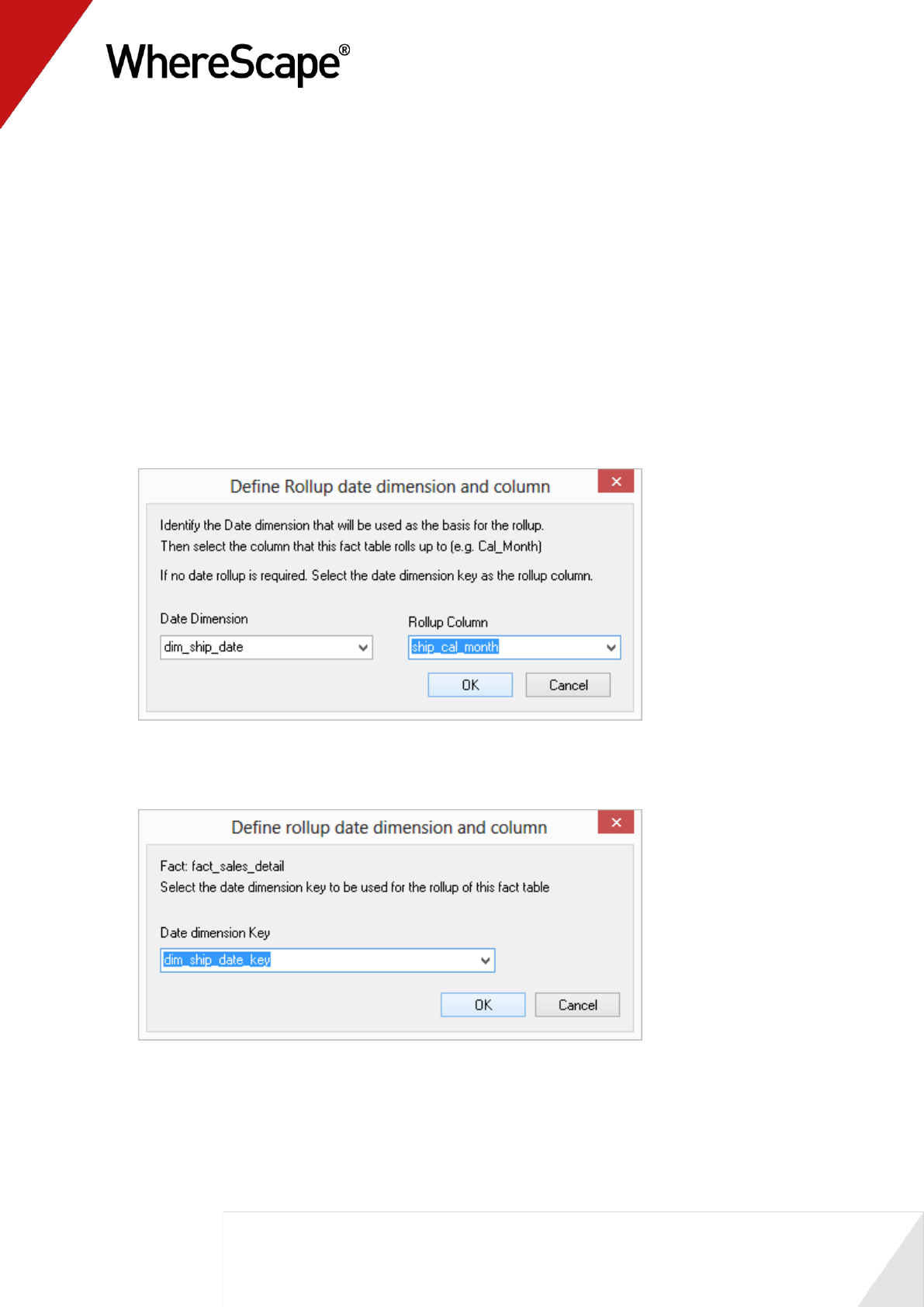
8 Rollup tables are rolled up via a dimensional hierarchy. You will be given the opportunity to
specify what to roll up on. From the dialog "Define rollup date dimension and column" select
the following then click OK.
Date dimension - dim_ship_date
Rollup column - ship_cal_month:
9 Now select the date dimension for each of the detail tables. For fact_sales_detail, choose
dim_ship_date_key and click OK.
93
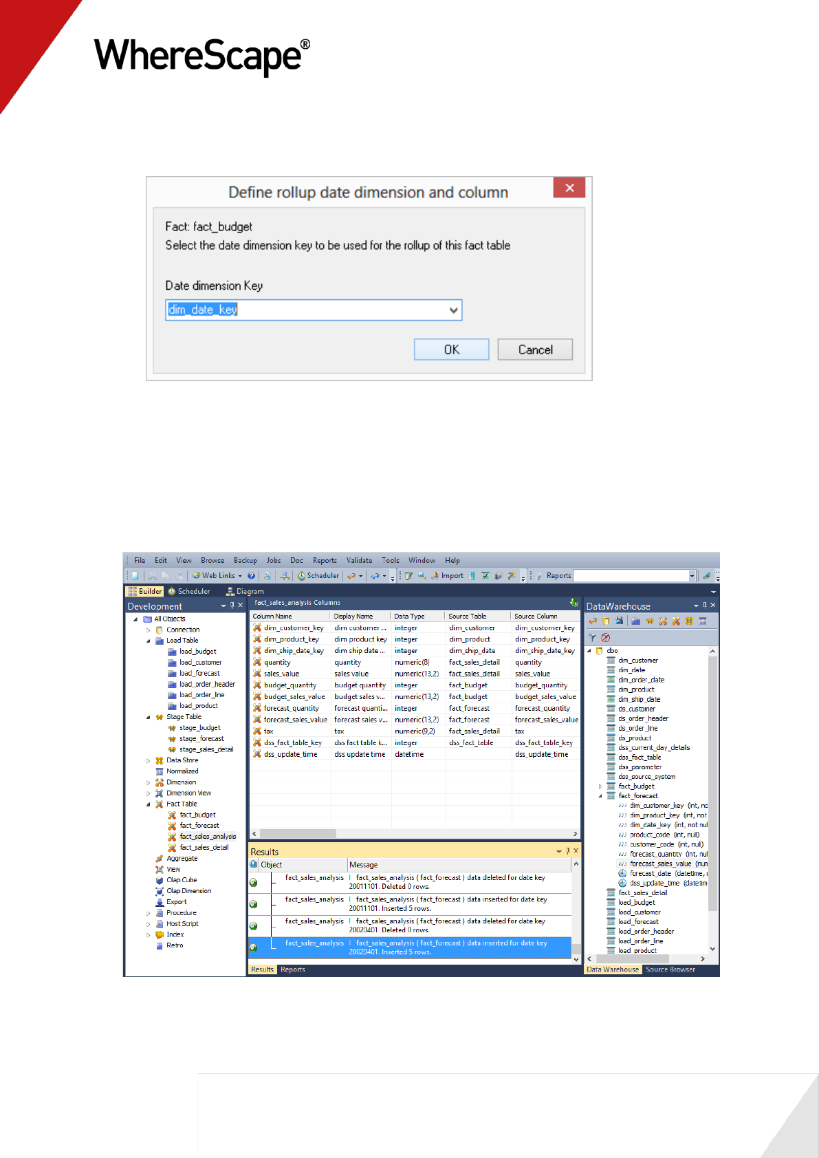
10 For fact_budget choose dim_date_key and click OK:
11 Finally for fact forecast again choose dim_date_key and click OK. This is required so
WhereScape RED knows which dimension to use to rollup each of these detail fact tables.
12 Populate the fact rollup table by right-clicking on fact_sales_analysis and choosing Execute
Update Procedure.
13 Your screen should look something like this:

95
2.7 Aggregate Tables
Aggregate tables are used to improve performance. They provide a subset of the main fact table
which the end user tools can navigate for a faster query time. An aggregate is typically created by
the deletion of items that don't make sense when summarized and by deleting one or more of the
dimension keys.
TIP: It is common practice to create two or more aggregate tables for large fact tables.
1 Double-click on the Aggregate object group in the left pane. Refresh the Data Warehouse
source table in the right pane (F5).
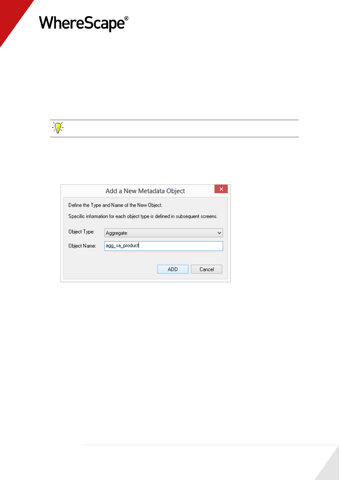
2 From the right pane drag fact_sales_analysis into the middle pane, changing the name to
agg_sa_product. Click ADD.
96
3 Click OK on the Properties dialog.
4 Click Close on the Create Database Table dialog.
5 Delete dss_fact_table_key so that data can be summarized from various source fact tables.
Also delete dim_customer_key and dss_update_time.
6 Create the aggregate table.
7 In the left pane right-click agg_sa_product and select Properties. Select (Build
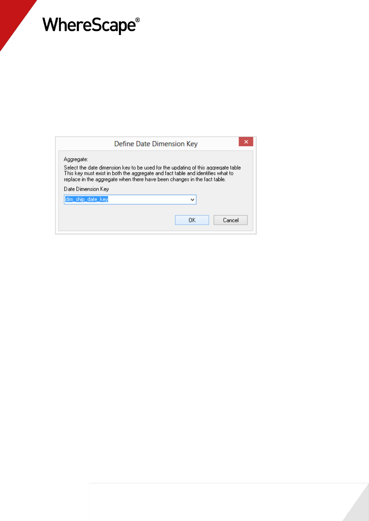
Procedure...) in the Update Procedure field and click OK on the Properties screen.
8 Select dim_ship_date_key as the date dimension key and click OK.
9 Update the table.
10 Refresh the Data Warehouse in the right pane (F5).
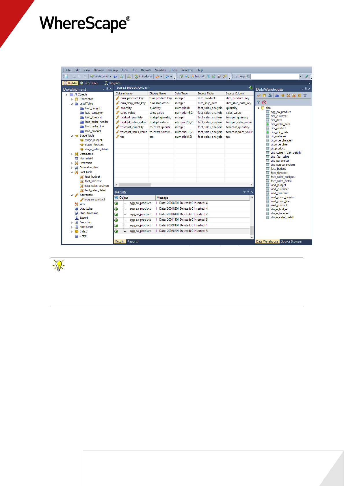
97
11 Your screen should look something like this:
TIP: For Oracle data warehouses. If you receive an "insufficient privileges" notification in
the Procedure Results, you need to grant the following privileges to the data warehouse user:
* Create materialized view
* Query rewrite
If you are unable to do this for any reason, contact your database administrator.
You are now ready to proceed to the next step - Creating a Customer Aggregate (see "2.8
Creating a Customer Aggregate" on page 98)
98
2.8 Creating a Customer Aggregate
This aggregate uses an alternative process to that described in Aggregate Tables. For this
process we will create a version of the product aggregate table's metadata and create a new
aggregate from this version.
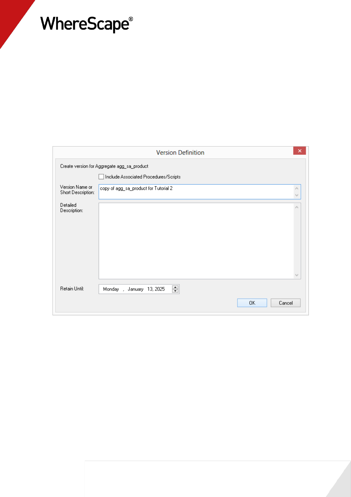
1 In the left pane, right-click on agg_sa_product and select Version Control / New Version.
2 The following screen displays. Enter a name for the new version and click OK.
99
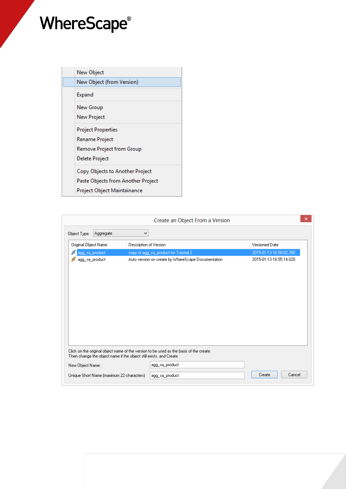
3 In the left pane, right-click on Aggregate and select New Object (from Version).
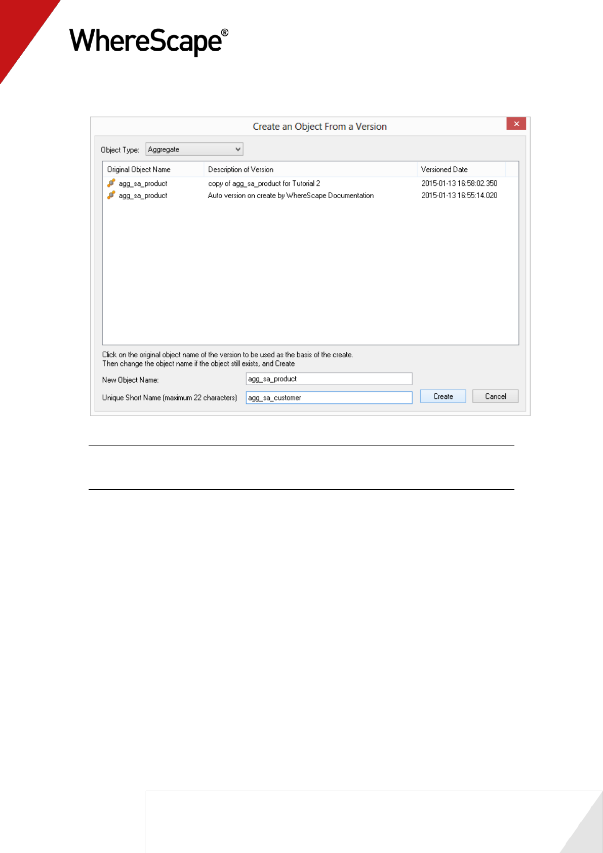
4 Double-click on the copy of agg_sa_product to select it.
100
5 Change the name and short name to agg_sa_customer. Click Create.
Note: Short names are used by WhereScape RED to derive names for associated objects (such
as index, procedures, cursor, etc). The table short name is limited in size to 22 characters in
Oracle and SQL Server and to twelve characters in DB2. It must be unique.
6 Select the new agg_sa_customer table in the left pane.
7 Delete the dim_product_key column, as this will be a customer and not a product based
aggregate.
8 Browse to the Data Warehouse and from the fact_sales_analysis table, drag
dim_customer_key into the middle pane.
9 In the left pane right-click agg_sa_customer and select Create (ReCreate).
10 In the left pane right-click agg_sa_customer and select Properties. For the Update Procedure
field select (Build Procedure...) and click OK.
11 Select dim_ship_date_key as the date dimension and click OK.
12 Right-click on the table in the left pane and select Execute Update Procedure.
13 Refresh the Data Warehouse in the right pane (F5).
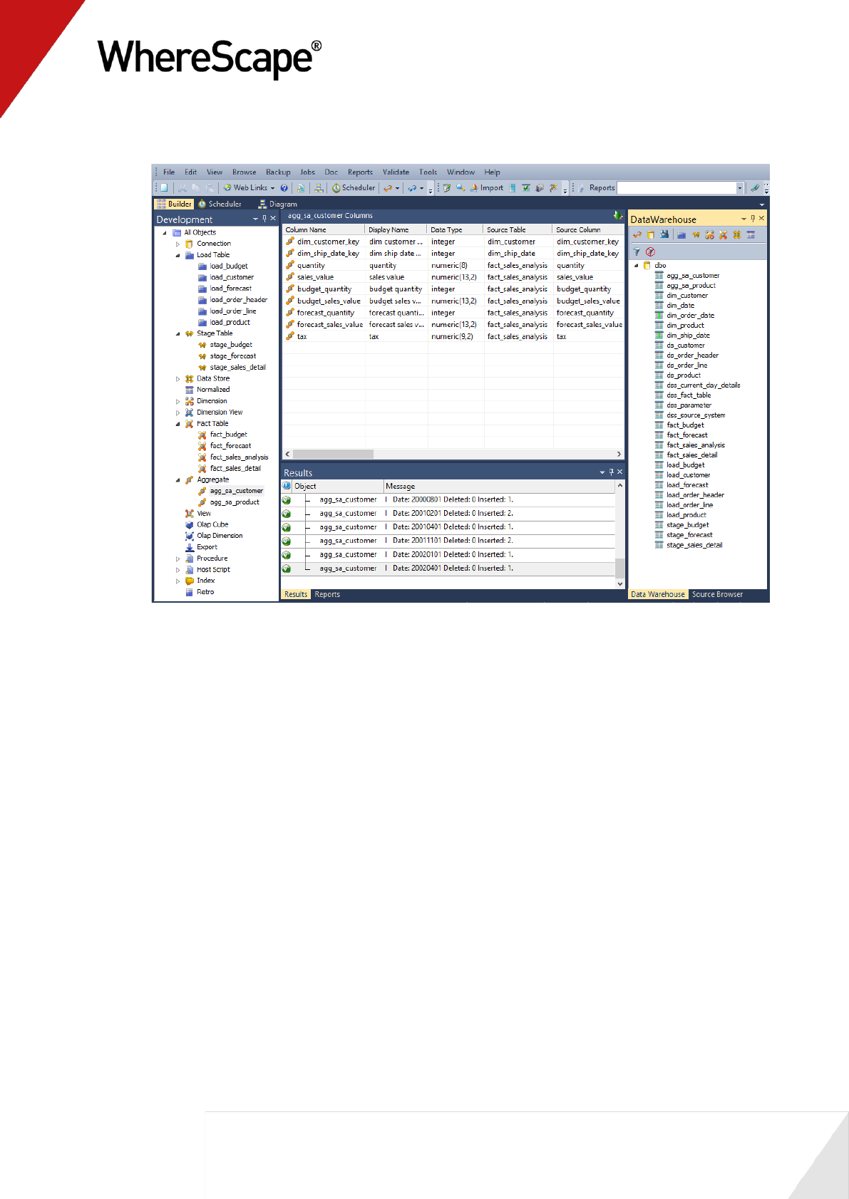
101
14 Your screen should look something like this:

102
Before you start on this chapter you should have:
Completed Tutorial 1 - Basic Star Schema Fact Table (see "Basic Star Schema Fact Table"
on page 1)
Successfully completed Creating a Fact Table (see "1.12 Creating a Fact Table" on page 58)
This chapter deals with the scheduling of the data warehouse objects created in the first tutorial.
We will cover the scheduling of a job and the editing of both the dependencies and the job.
In This Tutorial
3.1 Purpose and Roadmap .................................................. 103
3.2 Creating and Scheduling a Job ..................................... 105
3.3 Adding Tasks ................................................................ 106
3.4 Task Dependencies ....................................................... 109
3.5 Editing a Scheduled Job ................................................ 111
3.6 Job Results .................................................................... 113
3.7 Diagrammatic View for Jobs ......................................... 114
T u t o r i a l 3
Scheduling and Dependencies
103
3.1 Purpose and Roadmap
Purpose
The scheduler allows jobs (e.g. data loads and updates) to be run in background mode and/or at a
pre-determined time.
In this tutorial you will learn (i) how to set-up jobs and their associated job tasks (ii) create task
dependencies, and (iii) view job results.
This tutorial focuses on creating a job to update the fact_sales_detail star-schema created in
Tutorial 1.
Tutorial Environment
This tutorial has been completed using Oracle. All of the features illustrated in this tutorial are
available in SQL Server, Oracle and DB2 (unless otherwise stated). Any differences in usage of
WhereScape RED between these databases are highlighted.
Tutorial Roadmap
Step in Tutorial
Section
Create a new job for ‘Daily Update’.
Creating and Scheduling a Job
Add tasks to
Load load_customer
Load load_order_header
Load load_order_line
Load load_product
Update dim_customer
Update dim_date
Update dim_product
Update stage_sales_detail
Update fact_sales_detail
Analyze fact_sales_detail.
Creating and Scheduling Tasks
Setup task dependencies so that an analyze of
fact_sales_detail occurs after the table has
been updated.
Task Dependencies
Modify scheduling and runtime options (that
is, edit the job properties).
Editing a Scheduled Job
Check job results.
Job Results

105
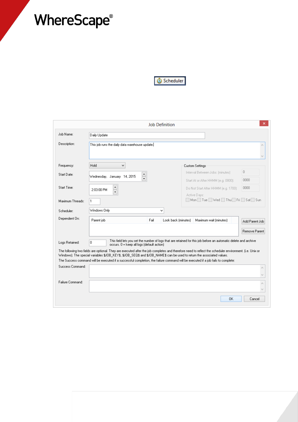
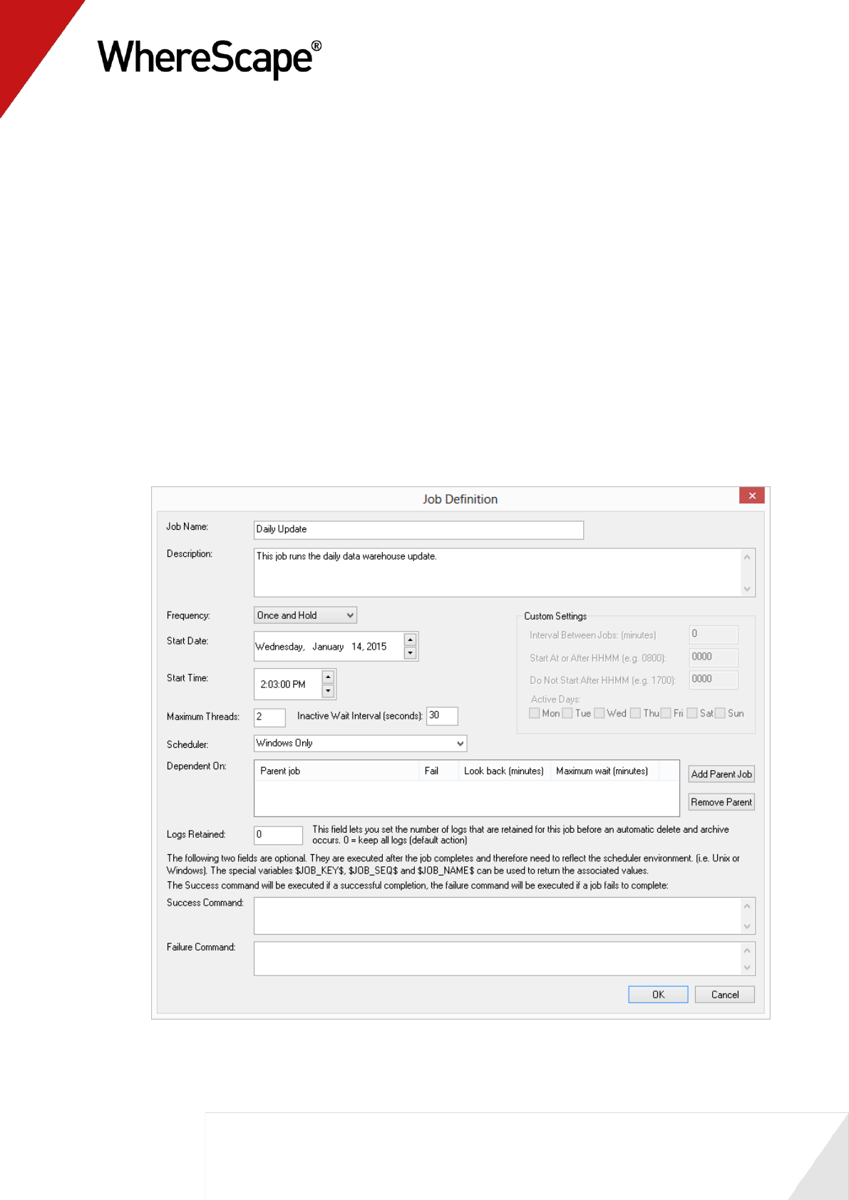
3.2 Creating and Scheduling a Job
To schedule a job click on the Scheduler button . This will open the scheduler
window. A new job can be initiated by selecting the File/New Job menu option.
The new job dialog will appear.
1 Change the job name to Daily Update and enter in the Description.
2 Click OK.
You are now ready to proceed to the next step - Adding Tasks (see "3.3 Adding Tasks" on page
106)
106
3.3 Adding Tasks
The task selection window contains an object tree in the left pane. Objects are selected from this
tree and added to the scheduled list of tasks in the right pane.
Perform the following actions to schedule an update of our fact table and dimensions.
1 Open the object tree by double-clicking on the All Objects project in the left pane.
2 Double-click on the Load Table object group.
3 Double-click on load_product, load_customer, load_order_line and load_order_header.
Note that as each object is double-clicked it is added to the right pane.
4 Double-click on the Dimension object group.
5 Double-click on dim_customer, dim_date and dim_product. As each object is double-clicked
it is added to the right pane. We do not add the date views since they do not alter, only the
underlying date dimension does.
6 Double-click on the Stage Table object group to expand it and then double-click on
stage_sales_detail to add this object to the right pane.
7 Double-click on the Fact Table object group to expand it and then double-click on
fact_sales_detail to add this object to the right pane.
8 Double-click again on fact_sales_detail to add a second copy of this object to the right pane.
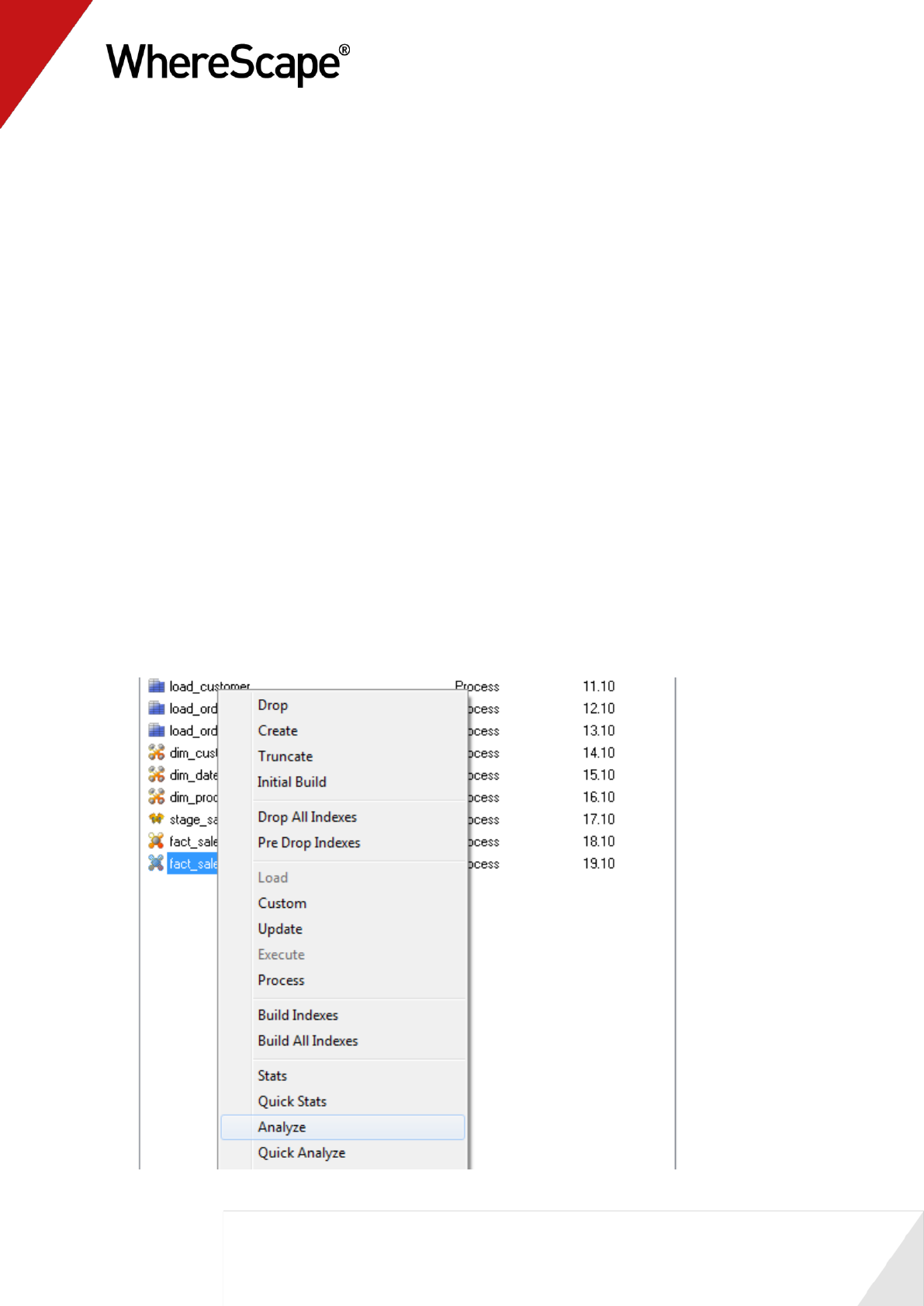
9 Right-click on the second fact_sales_detail and select Analyze.
107
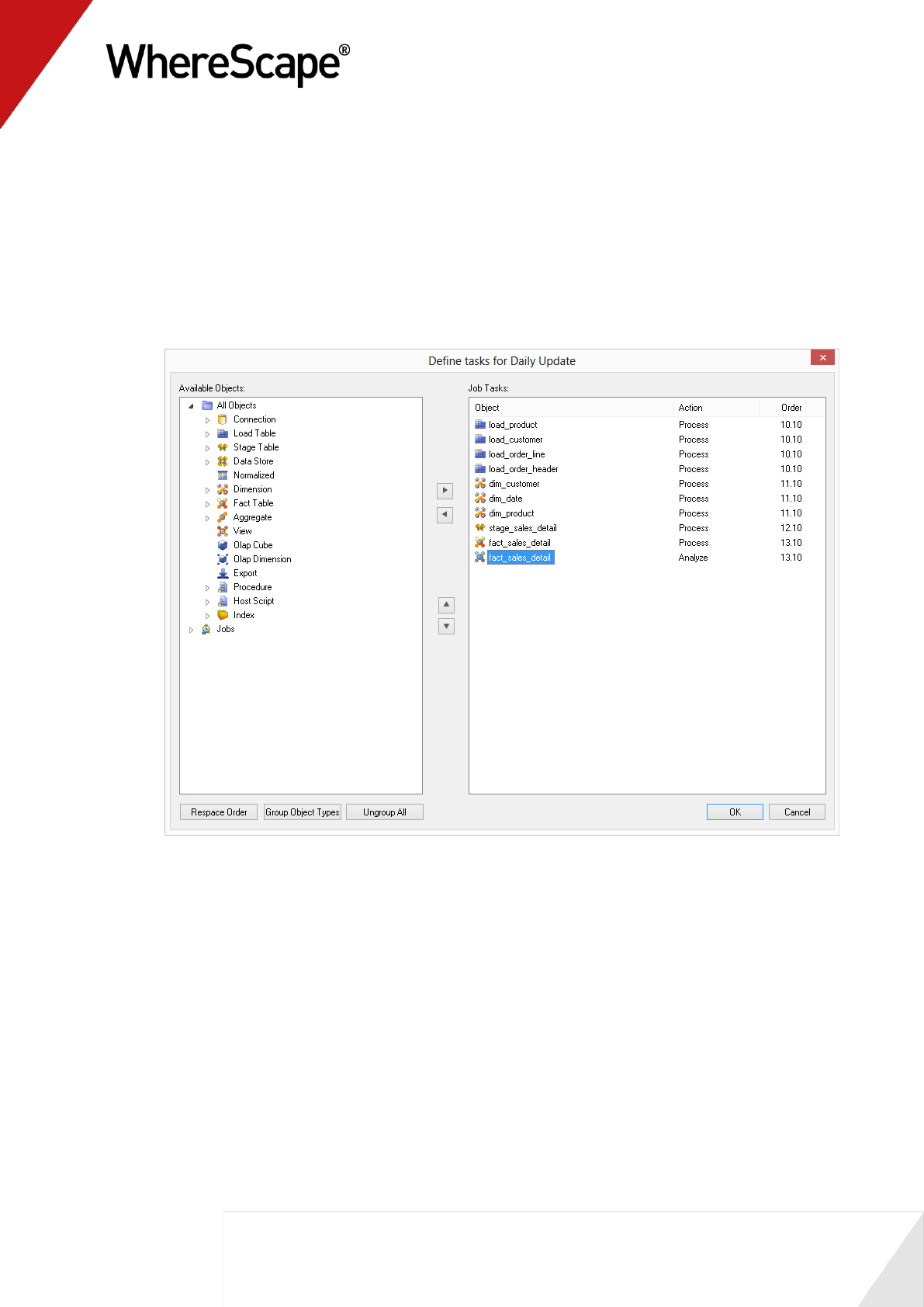
10 The 'Order' column defines the basic dependencies of the tasks. If the two numbers are the
same, then the tasks can run at the same time. In this example no tasks will run at the same
time. The job will process the tasks sequentially.
11 Click the Group Object Types button. You will notice that the order number for tasks of the
same type now have the same number. This will allow objects of the same type to run
concurrently. (i.e. all the load tables can be processed at the same time if there are sufficient
processing threads).
Your task selection window should now look like the following.
12 Notice that the tasks all have an action of Process with the exception of the last task which is
set to Analyze.|
The fact table fact_sales_detail has two actions. The first will process and update the table,
the second will analyze the table. At present these two actions can run at the same time. They
should however be sequential. We could alter the order of the second task by using the
right-click menu option Increase the Order. This would be the normal method, but we will
leave these two tasks with the same order and address the sequence of events in the next
section.

109
3.4 Task Dependencies
A scheduled job that is in a Hold or Waiting state can have its task dependencies altered. To
alter the dependencies for our newly defined job proceed as follows:
1 Click on the All Jobs button in the toolbar to display our Daily Update job in the top pane.
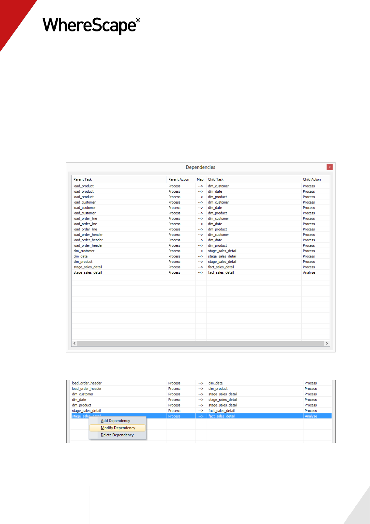
2 Position over the job name Daily Update and using the right-click pop-up menu select Edit
Dependencies. A list of the current task dependencies will be displayed. You will see that the
final two dependencies are from stage_sales_detail to each of the fact table tasks.
3 Right-click on the Parent task for the last dependency and select Modify Dependency.

110
4 Change the Parent task from stage_sales_detail (Process ) to fact_sales_detail (Process ).
Click OK to record the change. An example of this change is shown in the screen shot below.
5 Examine the new dependency list and see that the fact processing will now occur after the
stage processing and the fact analyze will occur after the fact processing.
6 Close the Dependencies dialog.
We are now ready to release the job, which is done in the next section - Editing a Scheduled Job
(see "3.5 Editing a Scheduled Job" on page 111).
111
3.5 Editing a Scheduled Job
Our job is now all set-up and ready to be released. We need to edit the job and change it from a
held job to one that the scheduler can action. Proceed as follows:
1 Click on the All Jobs button in the toolbar. Our daily update job will be displayed in the top
pane. Note that it is in an On Hold state.
2 Right-click on the job Daily Update and select Edit Job. The job definition screen will
re-appear.
3 Change the Frequency to Once and Hold. This will result in the job being run and then a
copy of the job being placed back in an 'On Hold' state so that it may be rescheduled for some
future processing. Note that other options exist under Frequency including 'Daily', 'Custom'
etc.
4 Change the Start Time to be 2 minutes from now.
5 Change the Max Threads counter to 2. This will allow two tasks to run concurrently. This
may not be a big help here, as the run should be very quick.
112
6 Click OK to save the changes.
7 Click on the All Jobs button in the toolbar. Our daily update job will be displayed in the top
pane. Note that its state should now be 'Waiting' or maybe 'Running'. If the job is in the
'Running' state we can double-click on the Job name to see the state of the individual tasks.
TIP: If you don't need to change a job and wish to run it immediately, select Start the
Job from the job's popup menu.
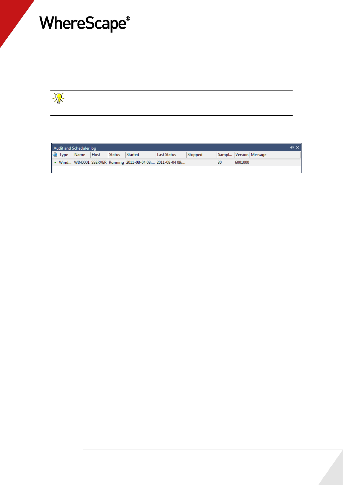
8 If the job does not go into a Running state after 30 seconds, check that a scheduler is running
by clicking on the Scheduler Status in the scheduler menu.
9 If no schedulers are running, refer to the Setup and Administration Guide on how to start a
scheduler.
We are now ready to proceed to the next section - Job Results (see "3.6 Job Results" on page 113)
113
3.6 Job Results
Once a job has completed, or in fact while it is running, we can check on the results of each of the
tasks by proceeding as follows:
1 Click on the All Jobs button in the toolbar. Our daily update job will be displayed in the top
pane. Note that if the job has started or is completed there will be two entries. One is in an
'On Hold' state and one is in a 'Completed', 'Running' or 'Failed' state.
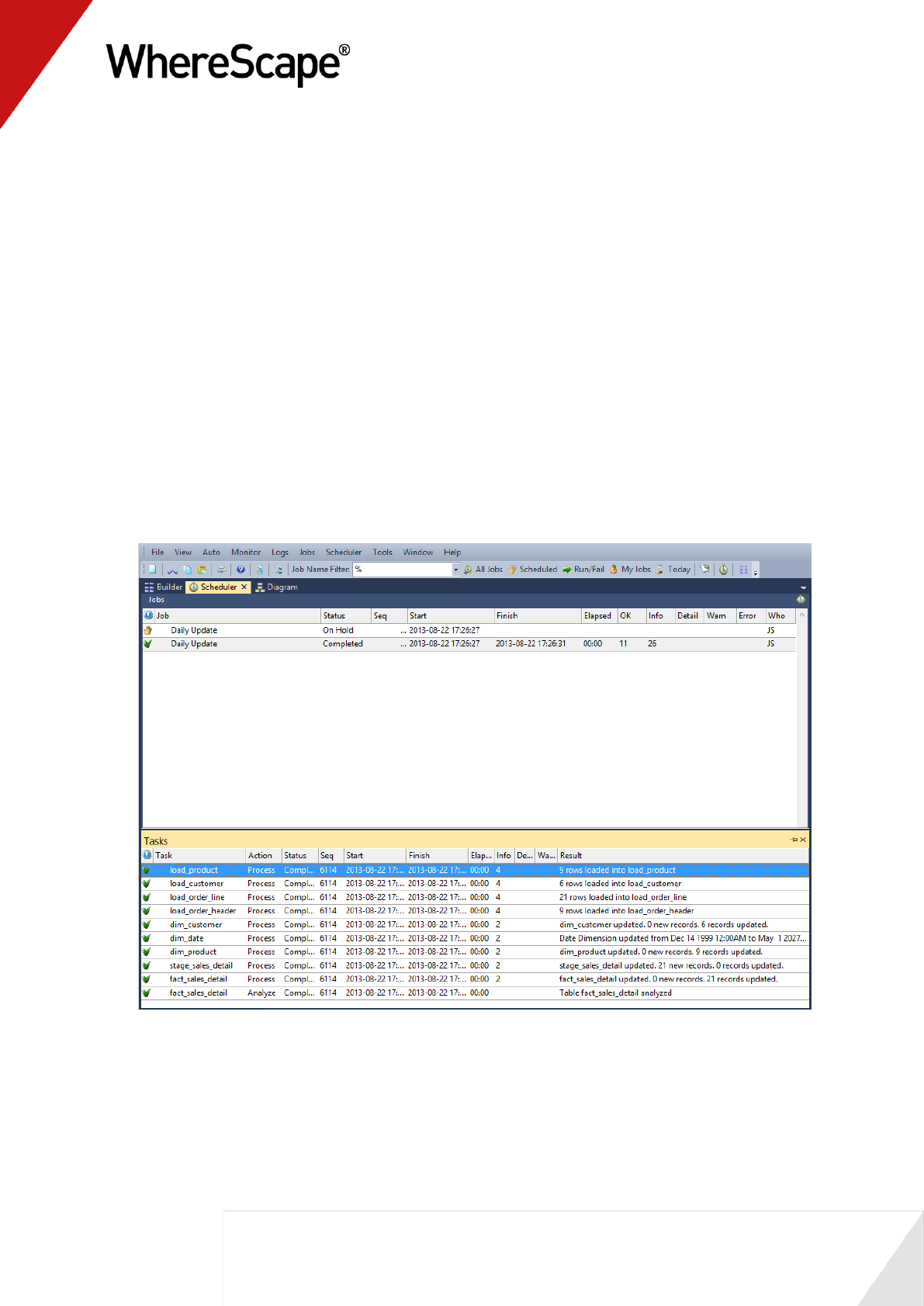
2 Double-click on the job Daily Update in a 'Completed', 'Running' or 'Failed' state to display
the individual tasks within the job.
3 Double-click on the fact_sales_detail task with action Process to display the messages
returned from this task. These messages should include information on any indexes dropped
and created.
4 Your screen should look something like this:
We are now ready to proceed to the next section - Diagrammatic View for Jobs (see "3.7
Diagrammatic View for Jobs" on page 114)
114
3.7 Diagrammatic View for Jobs
WhereScape RED provides the ability to diagrammatically view the job dependencies for the job
you have created.
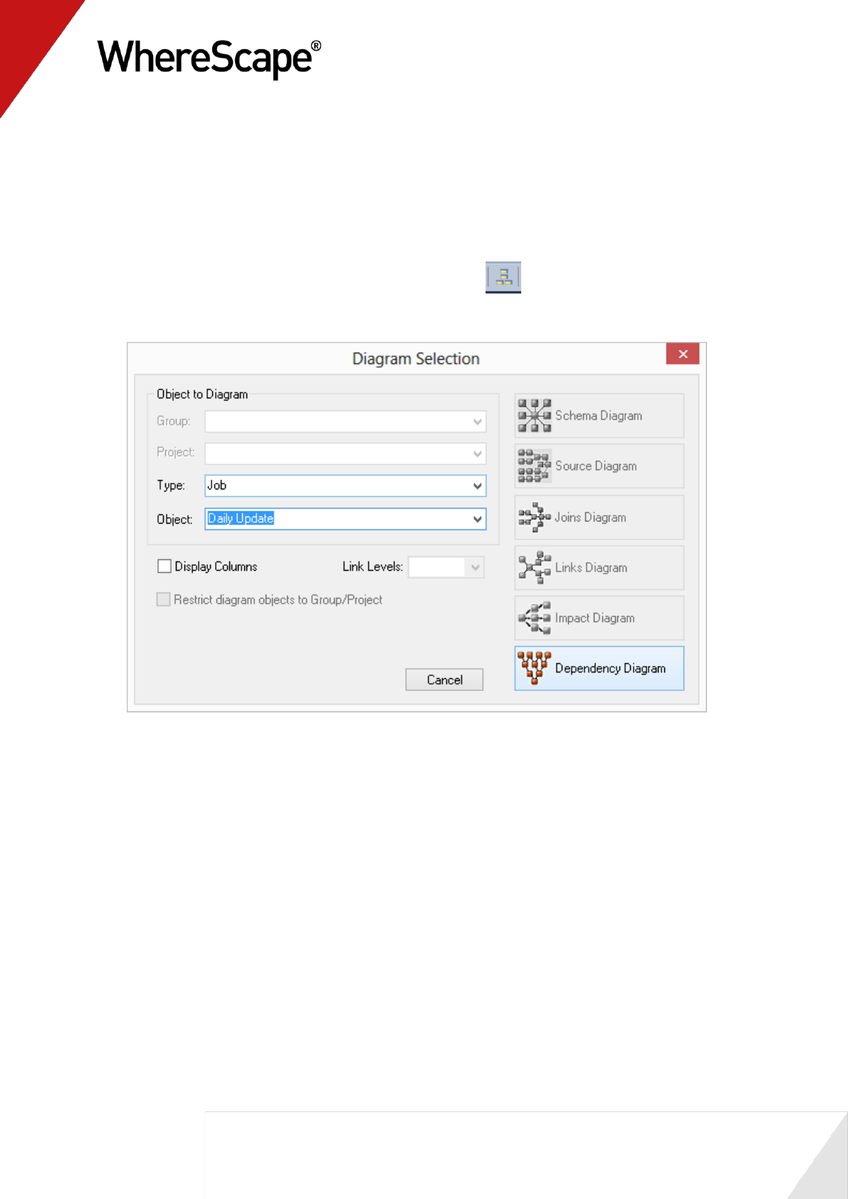
1 To bring up the Diagram Selection dialog, click on the button.
2 Select an object Type of Job to narrow the selection list and then select Daily Update. Click
on the Dependency Diagram button.
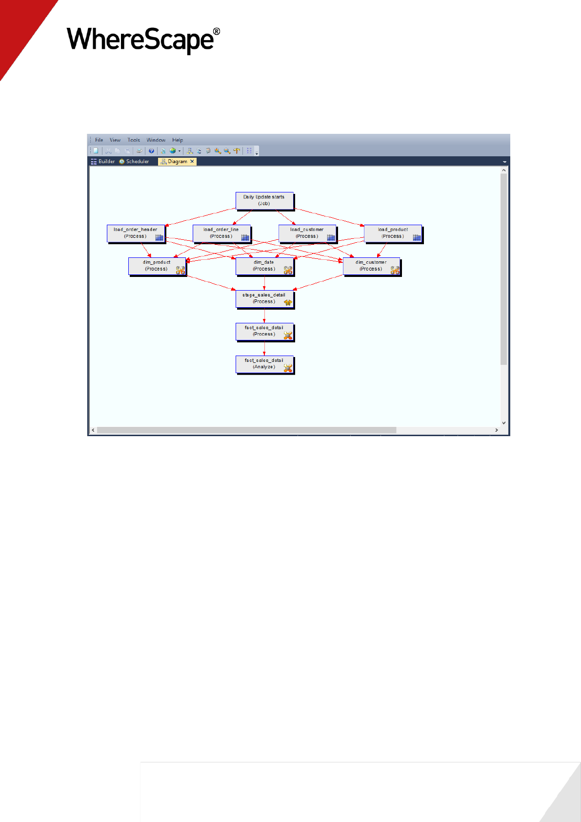
115
The diagram looks like this:

116
Before you start on this chapter you should have:
Completed Tutorial 1 - Basic Star Schema Fact Table (see "Basic Star Schema Fact Table"
on page 1)
Successfully completed Creating a Fact Table (see "1.12 Creating a Fact Table" on page 58)
This chapter deals with fine tuning the data warehouse by creating complex dimensions and
hierarchies.
In This Tutorial
4.1 Purpose and Roadmap .................................................. 117
4.2 Creating a Slowly Changing Dimension ....................... 118
4.3 Multiple Source Table Dimension ................................ 126
4.4 Creating a Dimension Hierarchy .................................. 136
T u t o r i a l 4
Complex Dimensions and Hierarchies
117
4.1 Purpose and Roadmap
Purpose
This tutorial will walk you through the process to:
Create a slowly changing dimension
Creating a complex dimension with multiple table sources
Adding hierarchies to a dimension for external maintenance and for use in Analysis Services
cubes.
In short, this tutorial alters the existing customer and product dimensions. The customer
dimension is converted to a slowly changing dimension and the product dimension has its
content enriched from additional data sources. Hierarchies are built on all dimensions that will
be used in the next tutorial.
Tutorial Environment
This tutorial has been completed using Oracle. All of the features illustrated in this tutorial are
available in SQL Server, Oracle and DB2 (unless otherwise stated). Any differences in usage of
WhereScape RED between these databases are highlighted.
Tutorial Roadmap
This tutorial works through a number of steps. These steps and the relevant section within the
chapter are summarized below to assist in guiding you through the tutorial.
Step in Tutorial
Section
Convert the customer dimension to a slowly
changing dimension.
Creating a slowly changing dimension
Add additional data sources to the product
dimension
Multiple source table dimension
Create hierarchies for the following tables:
dim_date
dim_customer
dim_product
Creating a dimension hierarchy
This tutorial starts with the section Creating a Slowly Changing Dimension (see "4.2 Creating a
Slowly Changing Dimension" on page 118)
118
4.2 Creating a Slowly Changing Dimension
The process of creating a slowly changing dimension is largely the same as creating a normal
dimension. Two additional questions are asked during the dimension creation process when the
'Slowly changing dimension' button is chosen during the dimension create. In this section we will
cover the more common scenario of changing an existing normal dimension to a slowly changing
dimension.
The dimension dim_customer created in tutorial one will be changed to a slowly changing
dimension.
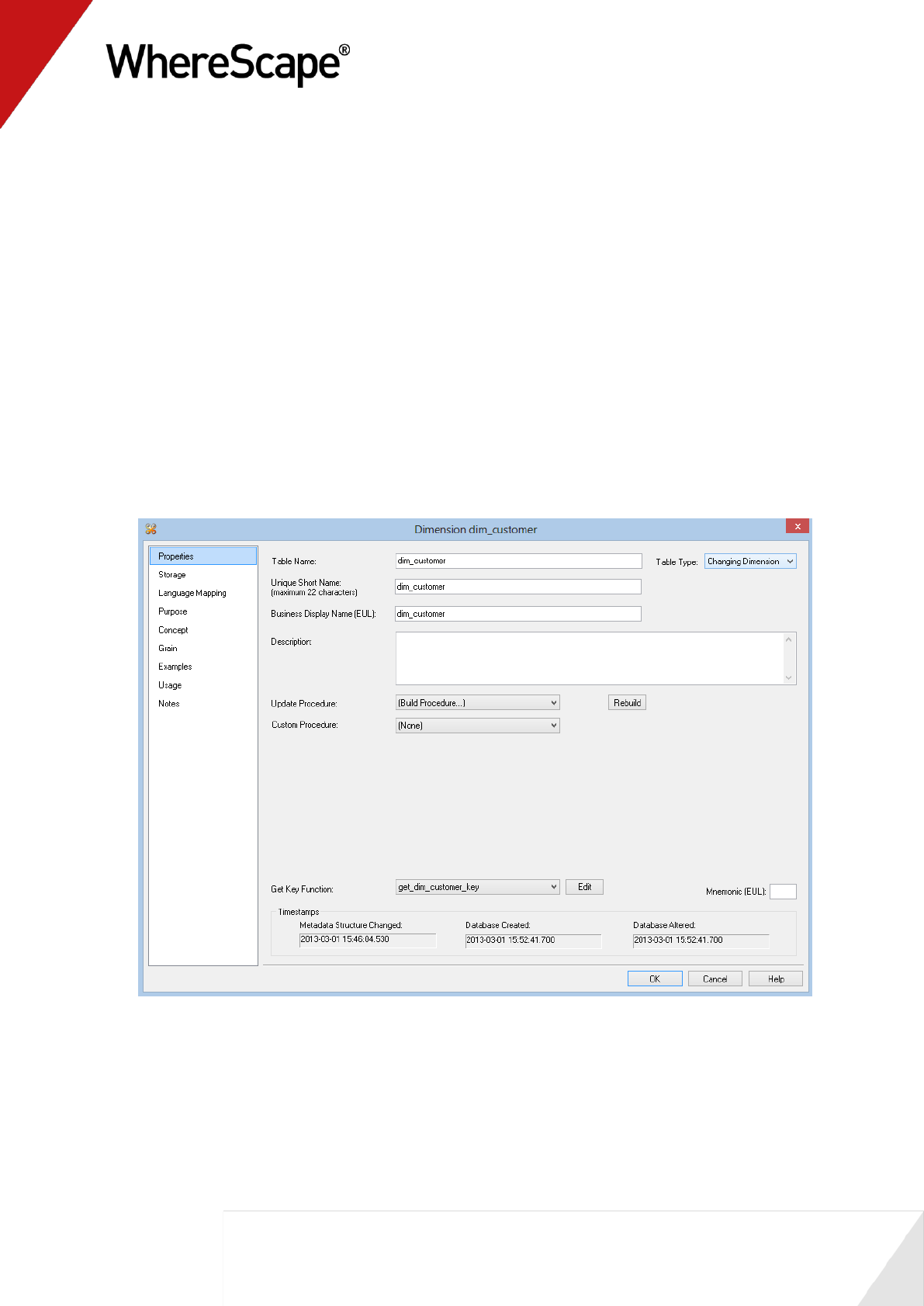
1 Right-click on dim_customer and select Properties.
2 On the dimension Properties change the Update Procedure drop-down to select (Build
Procedure...).
3 Use the Table Type drop-down to select Changing Dimension. Click OK.
119
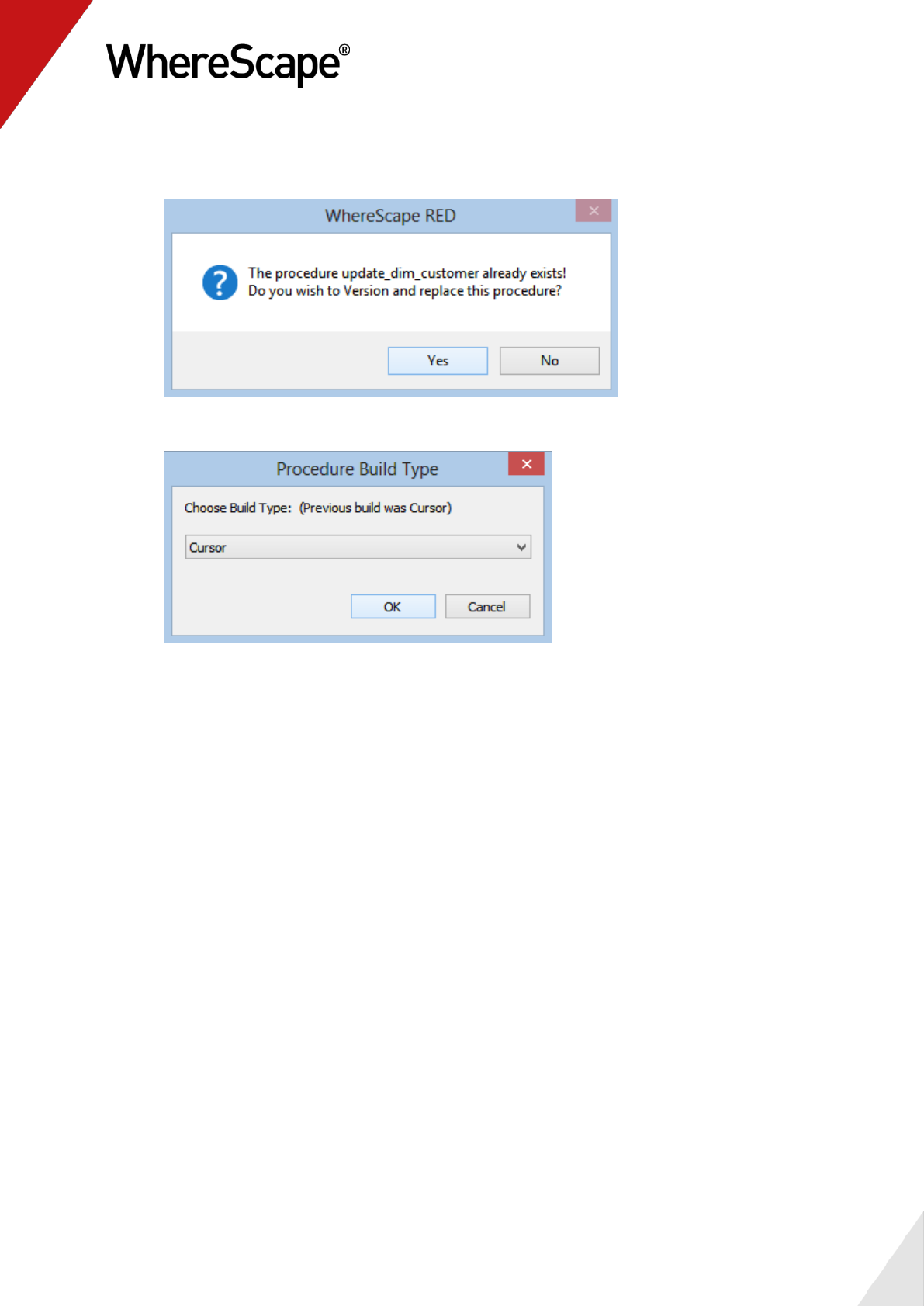
4 You will be asked if you wish to version and replace the update and get key procedures.
Answer Yes to both prompts.
5 A Procedure Build Type dialog will appear. Select Cursor.
120
6 The Define Dimension Business Key(s) dialog will be presented. The existing business key
code should already be the default value so click OK to proceed to the next screen.
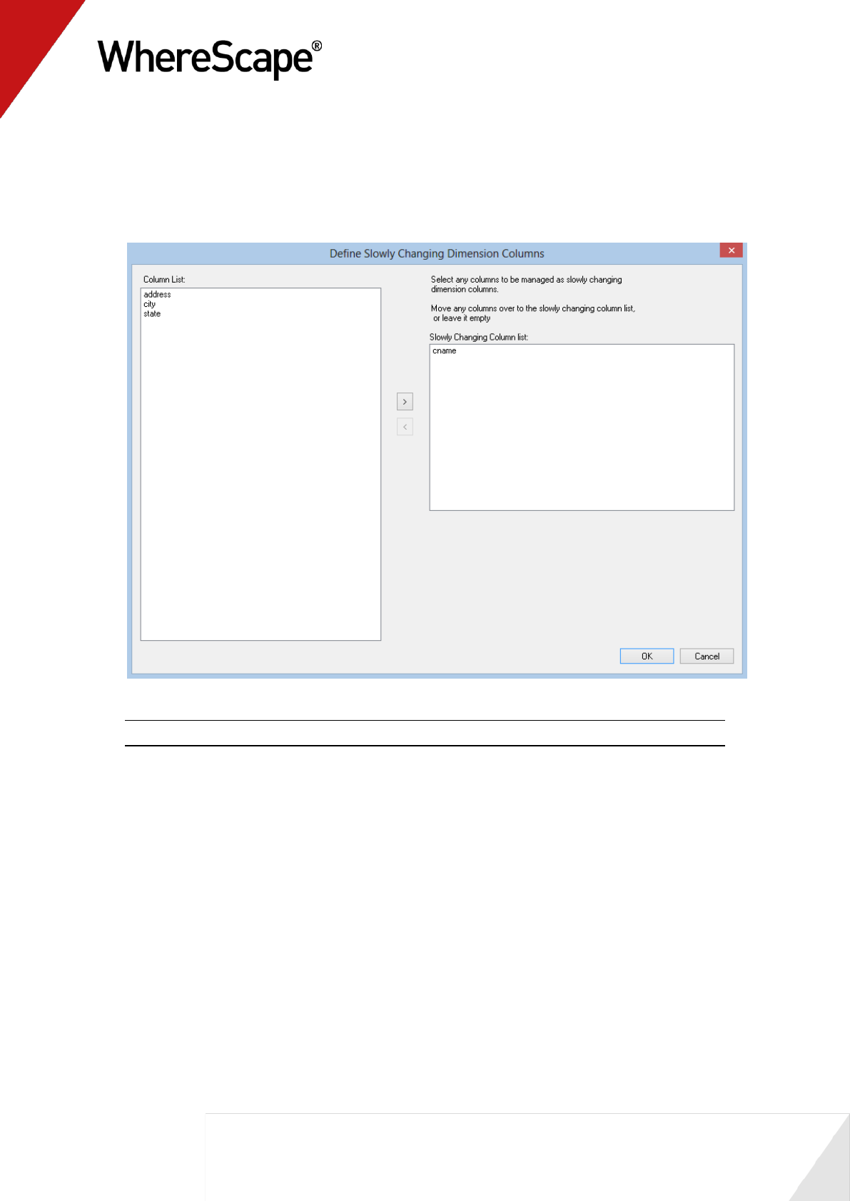
7 The Define Slowly Changing Dimension Columns dialog will now be presented. Multiple
columns can be selected to be handled as slowly changing. Double-click on cname to add it
to the list of slowly changing columns. Click OK.
Note: Refer to the Dimensions chapter for an explanation of slowly changing dimensions.
121
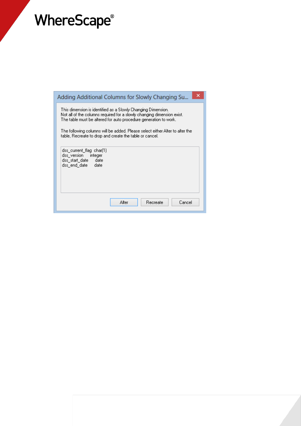
8 A dialog box will appear indicating that a number of additional columns will need to be added
to the dimension table in order to support a slowly changing model. The table can be Altered
(i.e. the columns added to the table) or re-created. As we have fact tables that use this
dimension we cannot re-create the table. To do so would make all of the joins in the fact
tables to this dimension invalid. Therefore we will alter the dimension. Click the Alter
button.
122
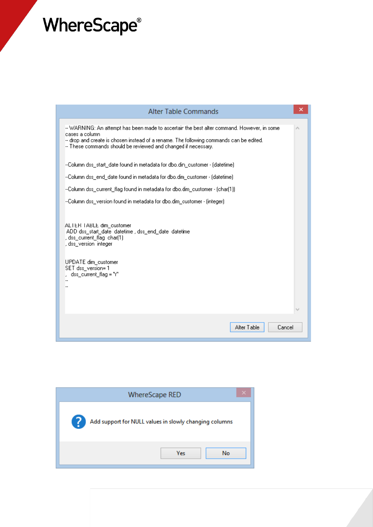
9 A dialog will now be presented with the SQL commands that will be executed to add the new
columns and set default values for the dss_version and dss_current_flag columns. Click the
Alter Table button to alter the table in the database. It is worth noting that whenever a
database table is altered from within WhereScape RED the SQL commands should be
reviewed. These commands can be changed if a different result is required.
10 A message box will appear informing you that the table was altered in the database. Click OK.
11 A dialog box will appear asking if you want to allow NULL support for the slowly changing
columns. The normal response would be No. Refer to the Dimensions chapter for a detailed
explanation. Click the No button.

123
12 The results dialog will show the indexes that were created/re-created for the dimension.
Note: There is a new index with a suffix of _SC to support the slowly changing dimension.
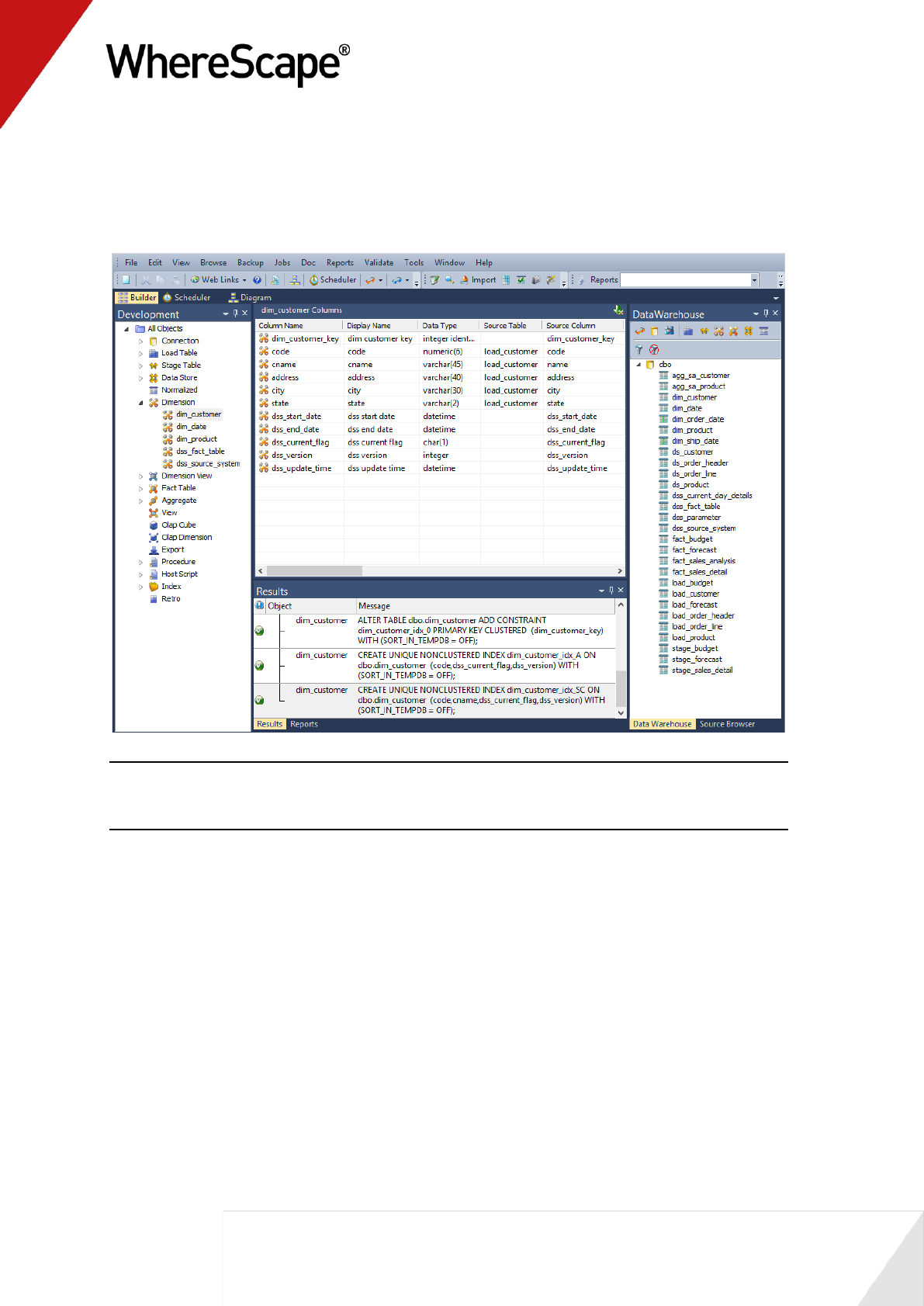
124
The dimension has now been converted to a slowly changing dimension. If a customer now has a
name change a new version of the customer record will be created to allow the tracking of the
customer by both the old and new name.
Your screen should look something like this:
Note: This conversion to a slowly changing dimension has changed the get key function for the
dimension. This function is called from the stage tables that use this dimension. We must now
rebuild the update procedures for the stage tables that use this dimension.
Rebuild Stage Update Procedures
As the customer dimension is used in the stage tables stage_sales_detail, stage_budget and
stage_forecast we will need to rebuild these procedures. Proceed as follows:
1 Right-click on stage_sales_detail and select Properties.
2 Use the Update procedure drop-down to select (Build Procedure...).
3 Click OK to leave the Properties page.
4 Answer Yes to the procedure versioning question.
5 Select Cursor for the procedure type.
6 Click OK on the Parameters dialog.
7 Click OK on the screen informing of multiple source tables.
8 Accept the previous entries by clicking OK on the cursor mapping screen.
9 Click OK on the business key join for each of the dimensions. The previously chosen business
key should be the default value provided.
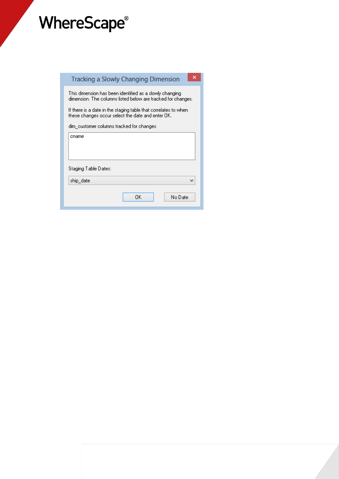
125
10 An additional dialog will appear after the customer dimension join. Select ship_date from the
date list and click OK.
11 Click OK on any other dimension joins.
12 Click OK on the business key for the stage table.
13 The update procedure will now be rebuilt to handle the fact that the customer dimension is
now slowly changing. Repeat steps (1) through (11) for the other stage tables stage_budget
and stage_forecast. Use the dates budget_date and forecast_date to track the dimension
changes.
You have successfully converted the dimension dim_customer to a slowly changing dimension,
and made all dependent changes.
You are now ready to proceed to the next section - Multiple Source Table Dimension (see "4.3
Multiple Source Table Dimension" on page 126).

126
4.3 Multiple Source Table Dimension
Dimensions typically get their information from multiple sources. A common scenario is to have
a series of codes that relate to the dimension. The descriptions of these codes are often stored in
a code lookup table. The following example will clarify the practice of producing a dimension
from multiple source tables.
The dimension dim_product created in tutorial one will be enhanced to provide additional
descriptions for the code values already present.
1 In the right pane, browse to the Tutorial connection that was created in tutorial one. Click
on the glasses or select the Browse/Source tables menu option. The tutorial tables should now
be shown in the right pane.
2 We need to acquire a number of additional source tables from the tutorial database.
Double-click on the Load Table object group in the left pane. This will list all the load tables
in the middle pane and make the middle pane a drop target for additional load tables.
3 Select the prod_group table from the right pane and holding the left mouse down drag to the
middle pane. Click ADD to add the new object and then OK on the Properties screen. Select
the Create and Load button.
4 Repeat steps (2) and (3) above to bring in and load from the prod_subgroup and prod_line
tables.
5 In the left pane click on dim_product. This will display all of the dimension columns in the
middle pane and make the middle pane a drop target for additional dimension columns. We
will be adding descriptions to it.
6 Browse to the Data Warehouse connection. The right pane should now show the data
warehouse tables. You can position the mouse in this right pane and select the menu option
'Filter - Load' to restrict the display to just load tables.
7 Expand load_prod_group, load_prod_subgroup and load_prod_line by double-clicking on
each table name.
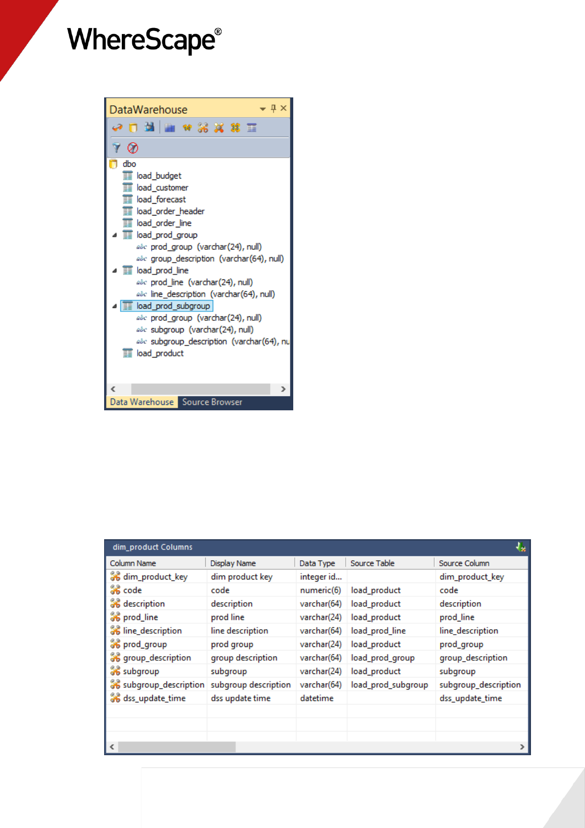
127
8 Drag group_description from load_prod_group into the middle pane. This will add it to the
product dimension columns.
9 Drag subgroup_description from load_prod_subgroup into the middle pane. This will add it
to the product dimension columns.
10 Drag line_description from load_prod_line into the middle pane. This will add it to the
product dimension columns.
11 Review the product columns displayed in the middle pane. Expand the 'source table' column
to see that we now have four different tables that contribute to the dimension.
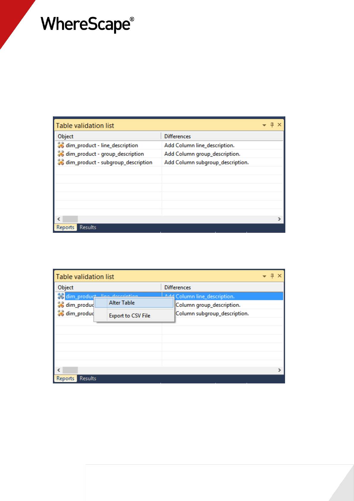
128
Right-click on dim_product in the left pane and select Validate against database. This
option will compare the metadata as displayed within WhereScape RED with the physical
table dim_product as it exists in the database. We have added new columns to the metadata in
the steps above, but the physical table has not been changed. A message will appear in the
middle pane as follows.
12 We now need to alter the physical table in the database. The message in the middle pane
shows that the metadata has additional columns not present in the dss table. Right-click on
dim_product in the middle pane and select Alter Table.
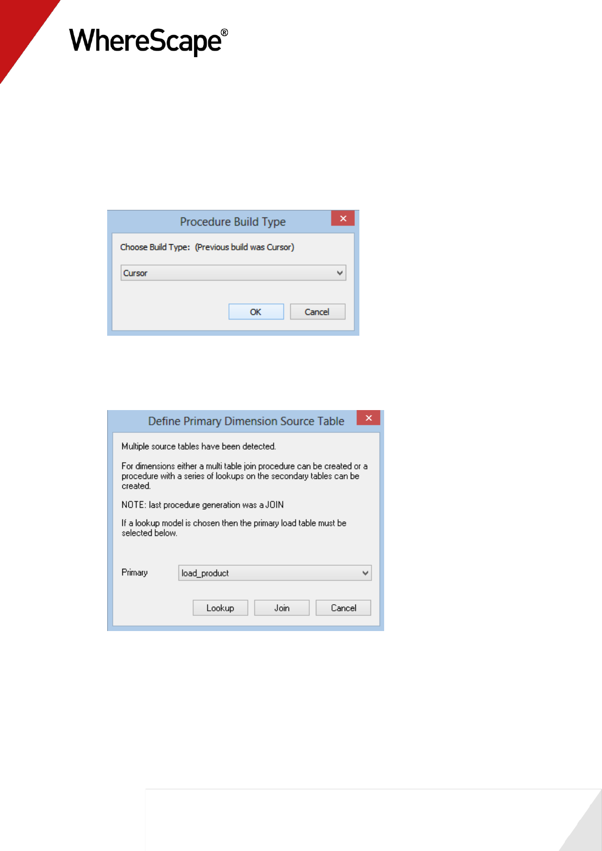
129
13 An alter table commands dialog will appear with the SQL commands that will be used to alter
the database table. Click the Alter Table button.
14 A message will display advising that the table was altered. Click OK to clear the message.
15 Repeat steps (12) to (14) for the other two changes.
16 Right-click on dim_product in the left pane and select Properties.
17 Click Rebuild.
18 A Procedure Build Type dialog will appear. Select Cursor.
19 A dialog will now appear asking you to define the primary source table and to choose between
a join of the source tables or a series of lookups. Refer to the Dimensions chapter for an
explanation on these two choices. The load_product should have been selected as the
primary source table. If it has not been selected then select it. Click the Lookup button.
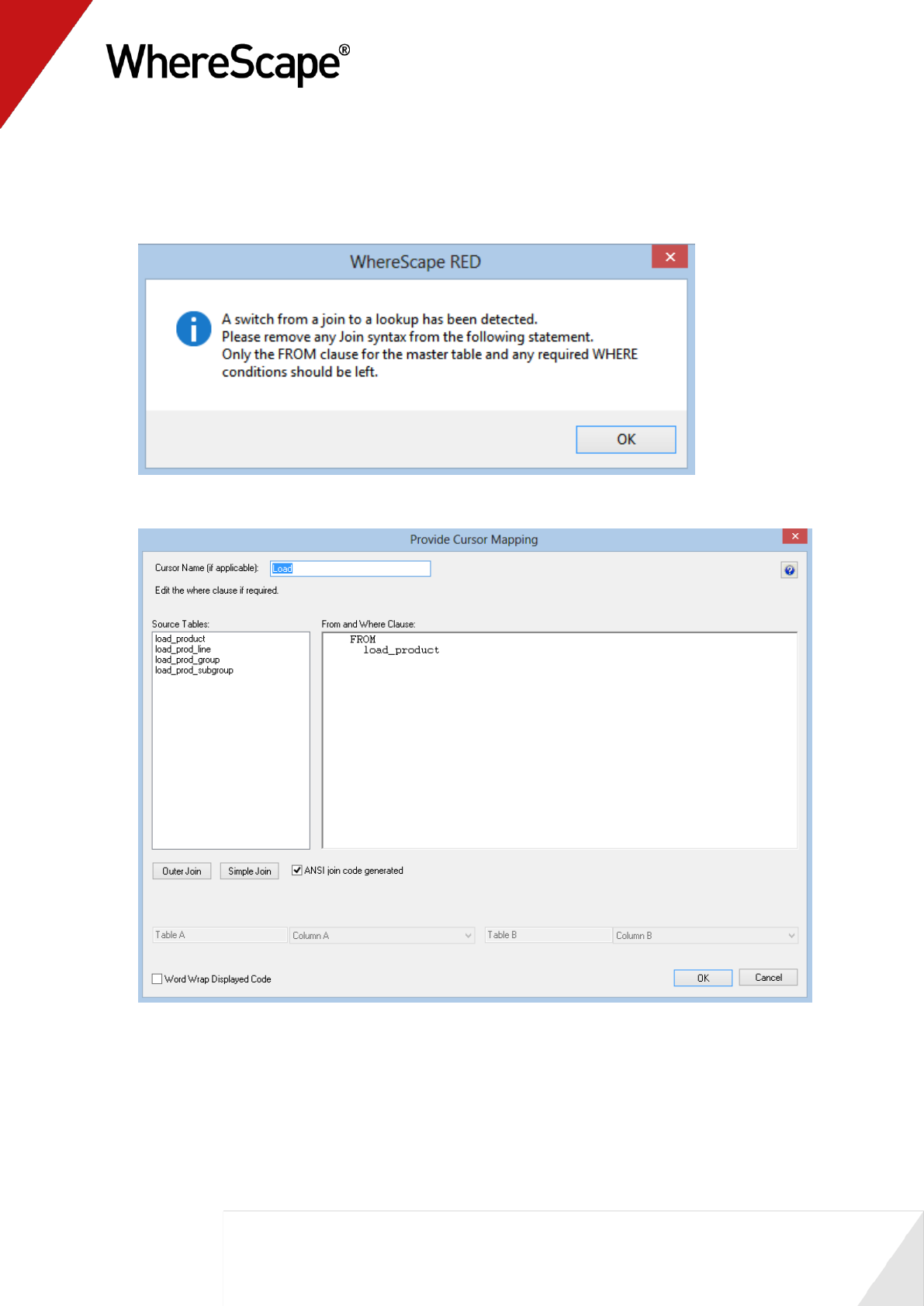
130
20 The Define Dimension Business Key(s) dialog will be presented. The existing business key
code should already be the default value so click OK to proceed to the next screen.
21 A message is displayed, asking you to ensure that any join syntax be removed from the
statement in the dialog to follow. Click OK.
22 Click OK on the Cursor Mapping screen.
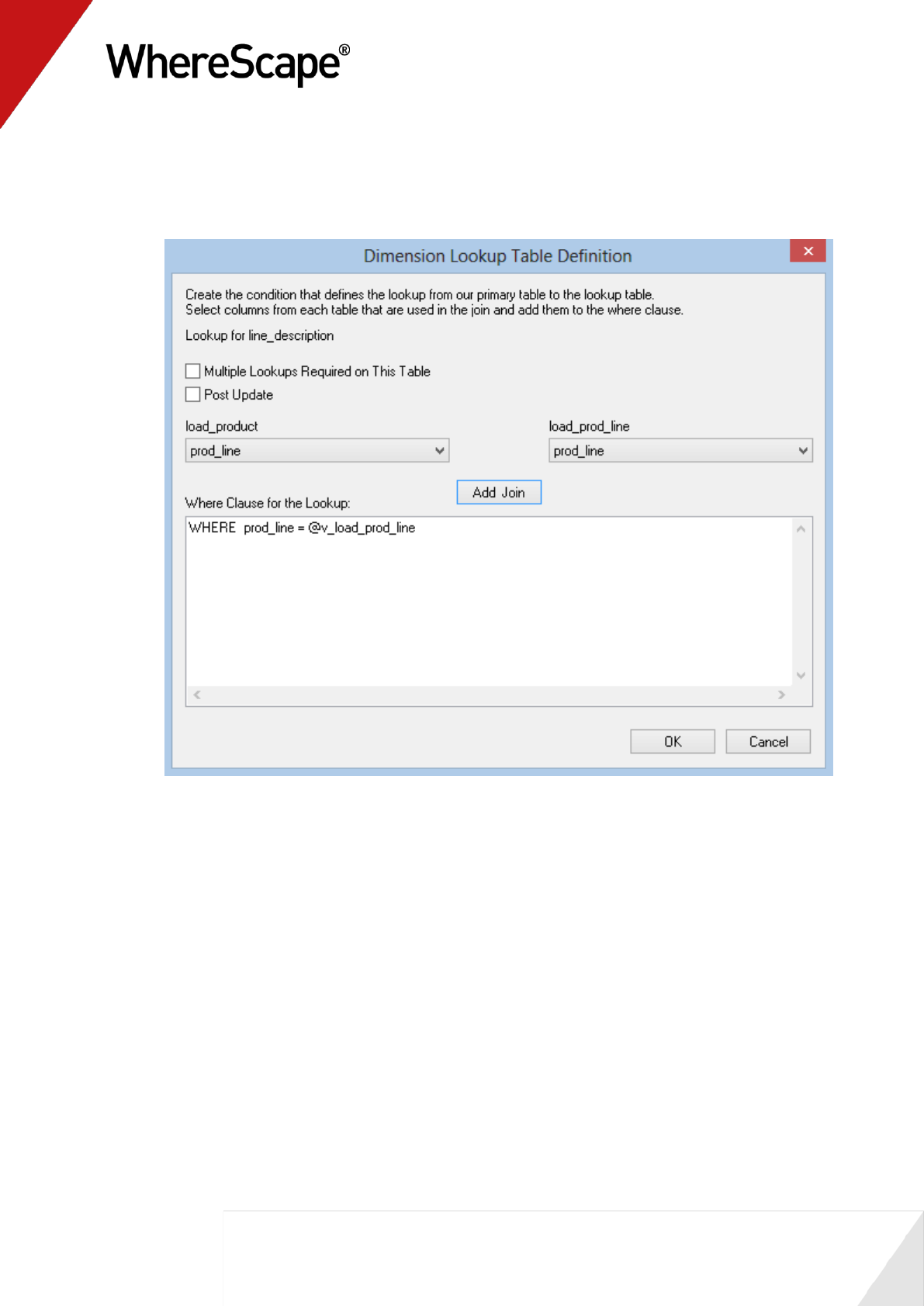
131
23 The Dimension lookup definition screen should now appear. Two drop-down boxes are
available. The left drop-down shows the columns for the table chosen as the primary source
table. The right drop-down shows the columns for the source table we wish to lookup. There
is a reminder above the left drop-down informing you which table is being looked up.
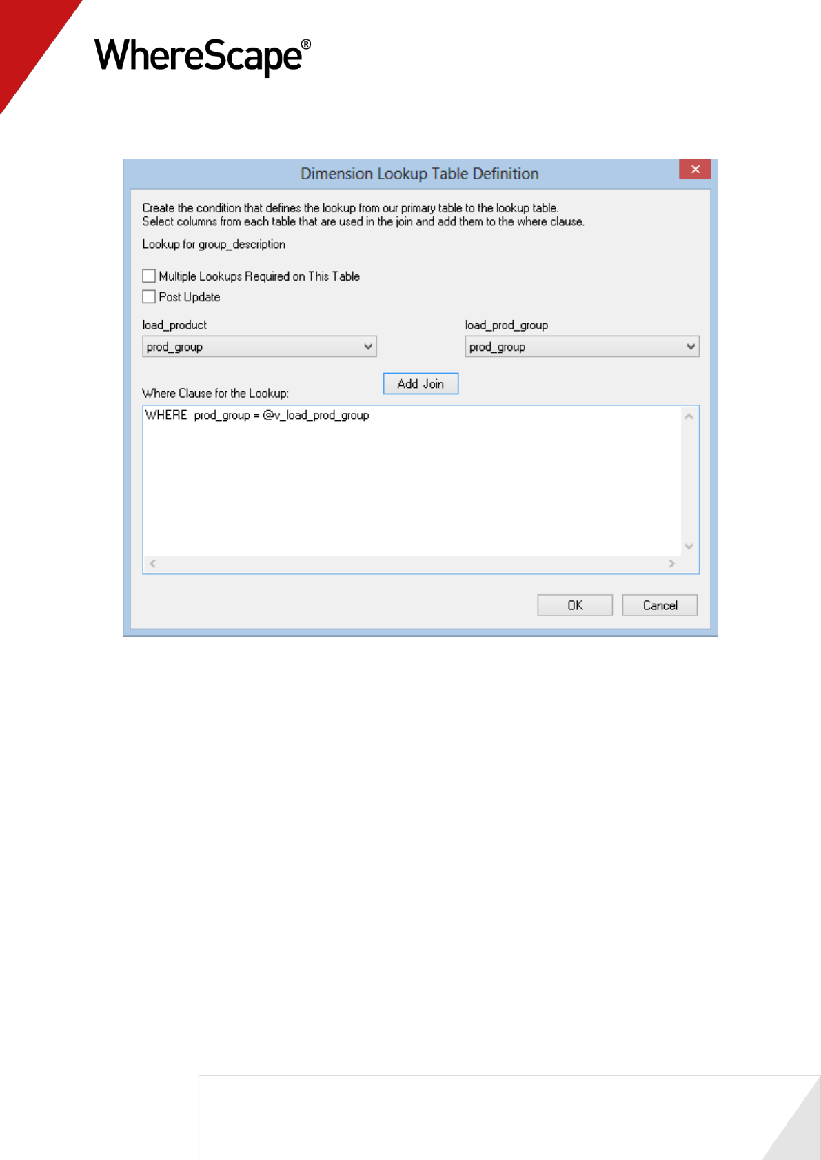
132
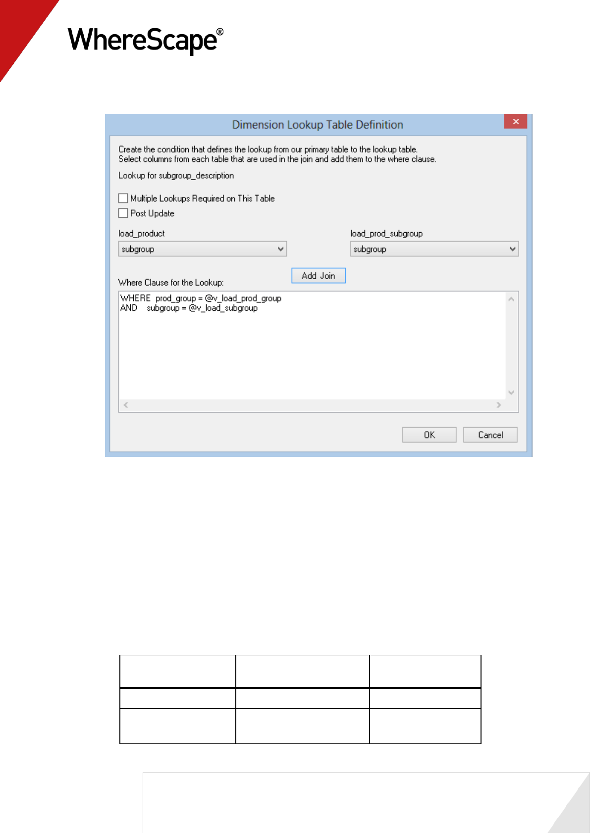
133
Although not being used at this point there are a number of features in these dialogs which
are worth noting. The first is that there is a checkbox to allow a table to be the source of
multiple lookups. This would be used where a generic code table was used to lookup
descriptions and we would need to make multiple lookups on the same table to get different
descriptions. The second is that procedure variables are available in the drop-down list of the
primary load table. Using this feature it is possible to make lookups that are dependent on the
results from previous lookups. This is done by selecting the columns that would have been
populated by the earlier lookups.
The lookups require that a join be defined for the two tables involved. The relevant joins for
our example are as follows. Step through the dialog boxes making these joins. First select the
column from each drop-down list and then click the Add Join button.
Lookup table
Primary src
(load_product)
Lookup column
load_prod_group
prod_group
prod_group
load_prod_subgroup
prod_group
prod_subgroup
prod_group
prod_subgroup
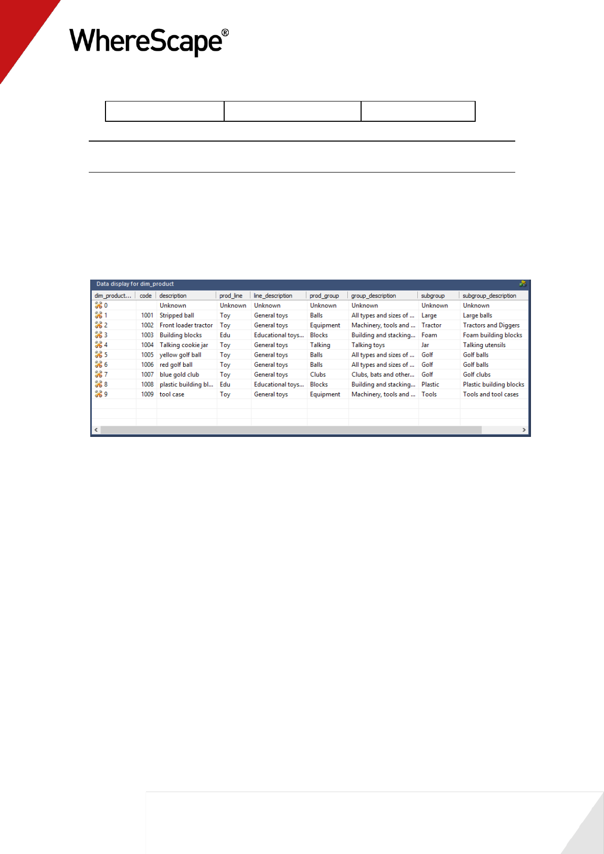
134
load_prod_line
prod_line
prod_line
Note: The load_prod_subgroup lookup will require two joins. After each join is made click the
OK button to move to the next dialog.
24 Once the lookups have been completed the procedure will be generated and the results dialog
will show the indexes that were created/re-created.
25 Right-click on dim_product in the left pane and select Execute Update Procedure. The
dimension will now be refreshed.
26 Right-click on dim_product in the left pane and select Display Data. Provided the lookups
were done correctly, the descriptions should now be populated.
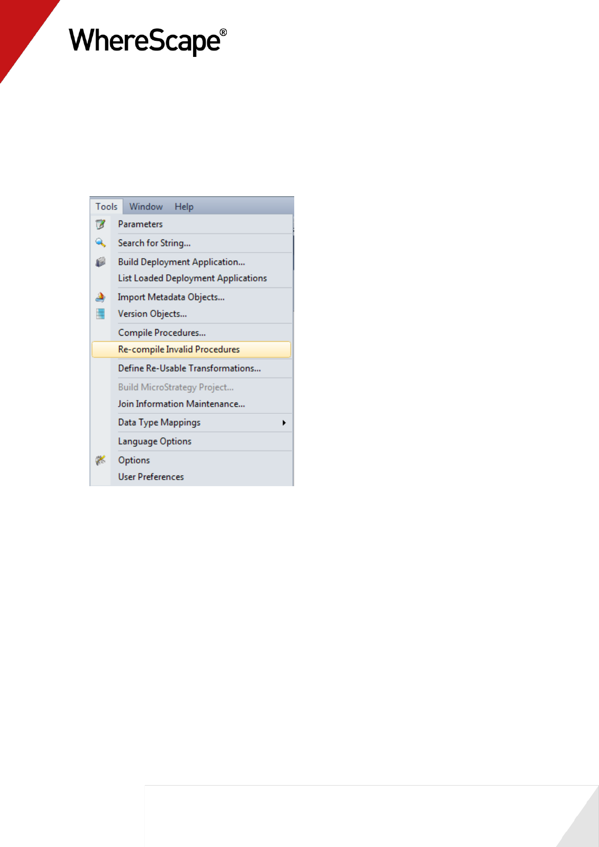
135
Oracle Procedure Invalidation
If running this as a tutorial in an Oracle Data Warehouse then the procedures
update_stage_sales_detail, update_stage_budget and update_stage_forecast will have been
invalidated. These procedures all use the function get_dim_product_key. This function was
re-compiled as part of the process above, but has not changed in structure.
Select the menu option Tools/Re-compile Invalid Procedures:
Click Yes to proceed. The three procedures will be re-validated and the results shown in the
middle pane.
You are now ready to proceed to the next section - Creating a Dimension Hierarchy (see "4.4
Creating a Dimension Hierarchy" on page 136)
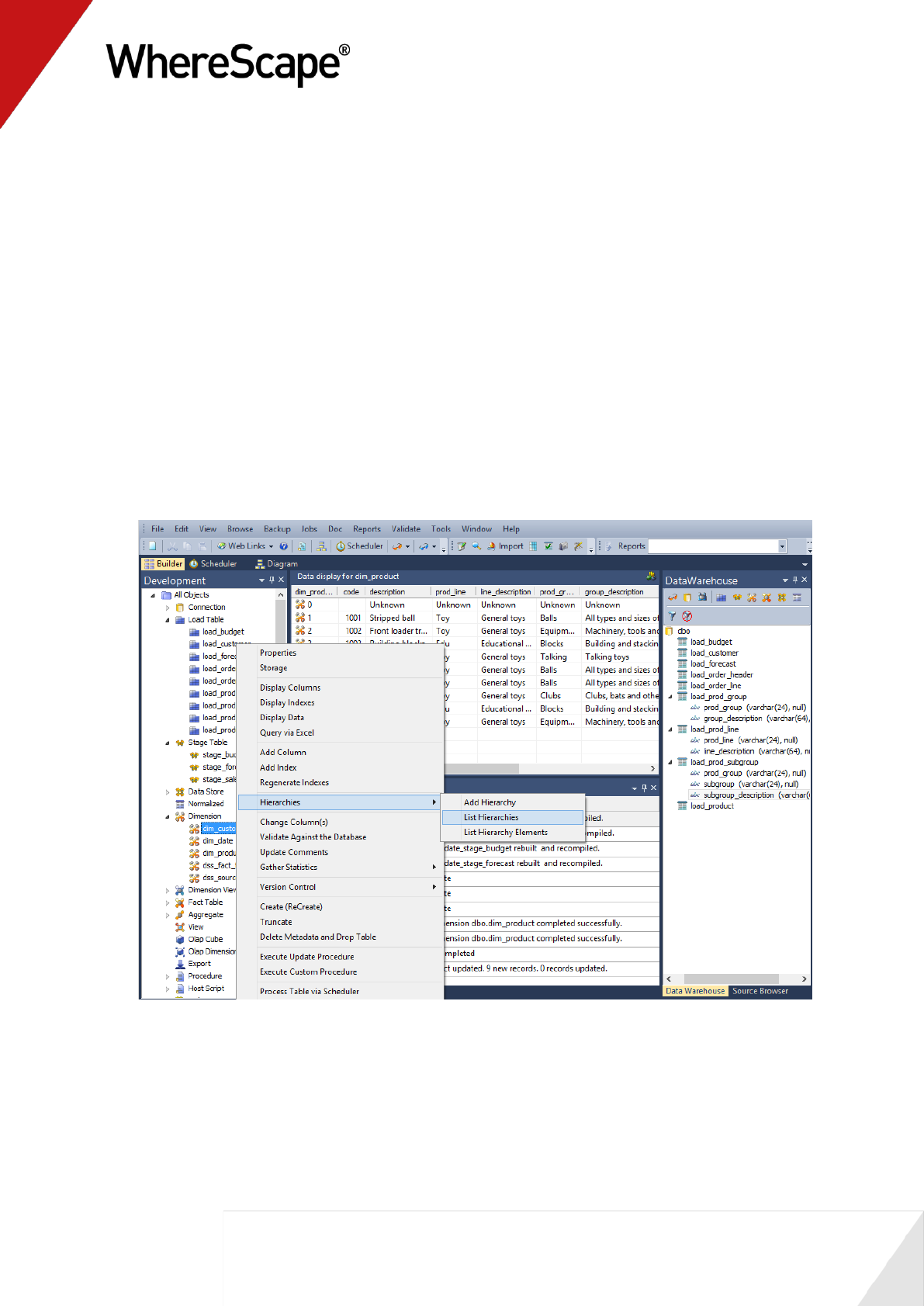
136
4.4 Creating a Dimension Hierarchy
Dimensions often have a number of hierarchical levels. An example is the date dimension which
has a natural hierarchy of year, month and day. WhereScape RED allows the definition of a
hierarchy against a dimension. A dimension may have multiple hierarchies defined. These
dimension hierarchies are used in the generation of Analysis Services cubes. Every dimension in a
cube must have a hierarchy with at least one element in it. Hierarchies can also be accessed and
the underlying data maintained with the Hierarchy maintenance utility shipped with the
enterprise version of WhereScape RED. This utility allows a user to maintain a hierarchy structure
in a different database or schema so that the data warehouse can use this structure as input to the
dimension. See the hierarchy section in the Dimension chapter for more details.
We will add a hierarchy to the dimensions dim_product and dim_customer created in the first
tutorial. We will also check that a hierarchy exists for the date dimension and if not present, add
one.
1 Right-click on dim_customer in the left pane and select Hierarchies / List Hierarchies.
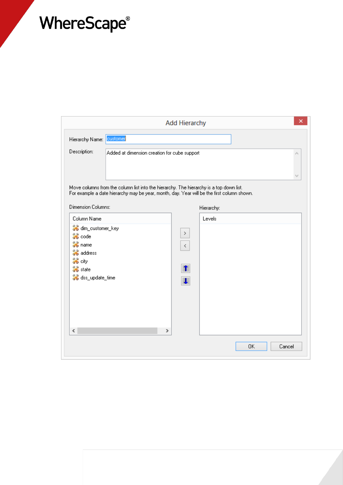
137
2 A list of any existing hierarchies will be shown in the middle pane. Initially there are no
hierarchies defined.
3 Right-click on dim_customer in the left pane and select Hierarchies / Add Hierarchy.
4 A dialog will appear asking for a hierarchy name and the hierarchy elements. Enter customer
for the name and add state, city, address and code as hierarchy elements.
5 Enter a meaningful Description for the hierarchy and click OK to exit the add hierarchy
dialog.
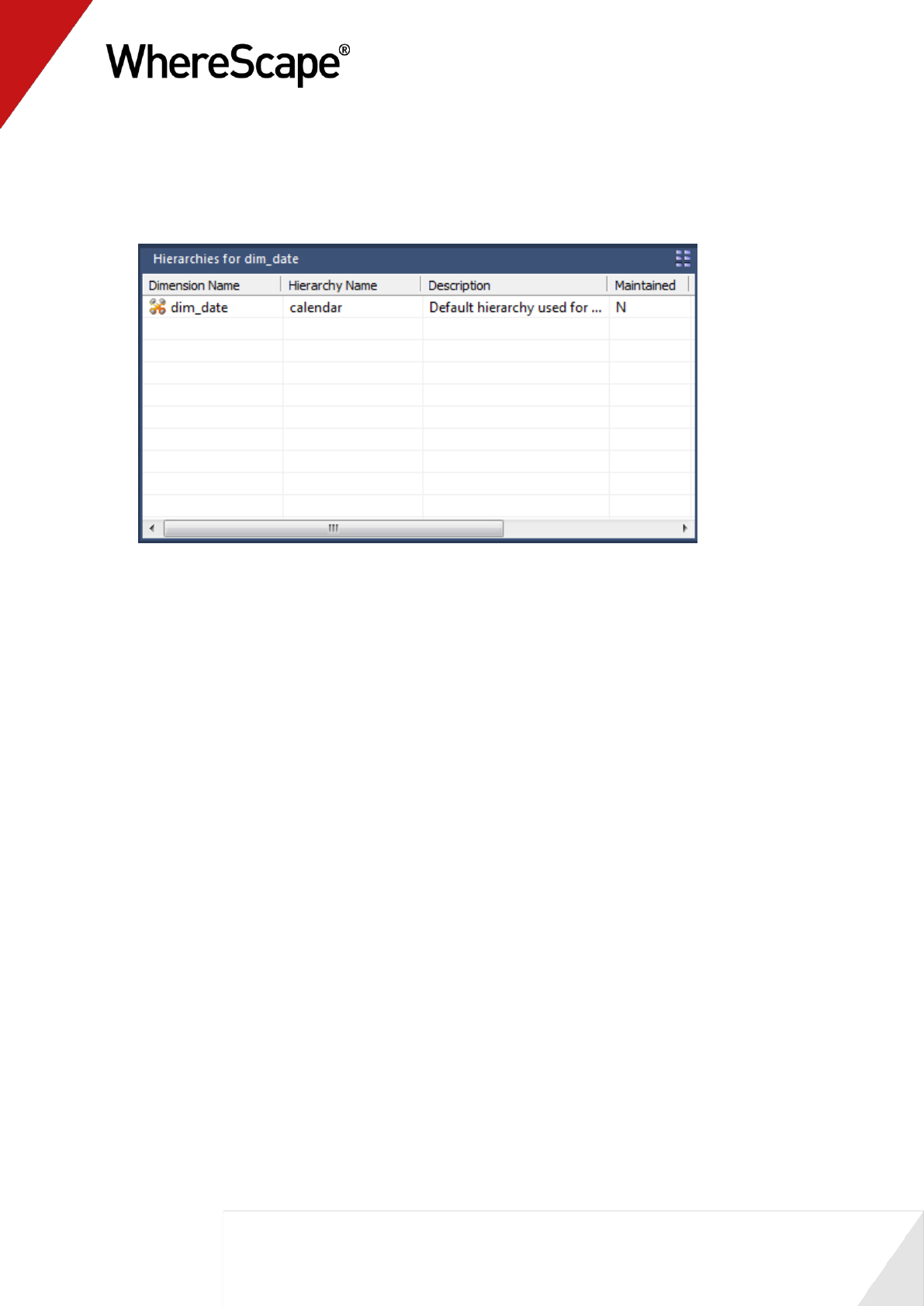
138
6 Repeat steps (1) through (4) for dim_product defining a top down hierarchy of
line_description, then group_description, subgroup_description, and code.
7 Check to see if a hierarchy exists for dim_date. If no hierarchy exists then add a top down
hierarchy of cal_year, cal_month and calendar_date.
As mentioned above these hierarchies are utilized by other processes within the data warehouse.
In this case we will use the hierarchies created in the building of Analysis Services cubes in the
next tutorial.

139
Before you start on this chapter you should have:
Completed Tutorial 1 - Basic Star Schema Fact Table (see "Basic Star Schema Fact Table"
on page 1)
Completed Tutorial 2 - Rollup Fact Tables, ASCII File Loads, Aggregates (see "Rollup Fact
Tables, ASCII File Loads, Aggregates" on page 73)
Completed Tutorial 4 - Complex Dimensions and Hierarchies (see "Complex Dimensions and
Hierarchies" on page 116)
This chapter deals with fine tuning the data warehouse by adding Analysis Services cubes.
In This Tutorial
5.1 Purpose and Roadmap.................................................. 140
5.2 Creating an OLAP Cube Object .................................... 141
5.3 Adding a Measure Group .............................................. 170
5.4 Cube Connections for Other Databases ....................... 184
T u t o r i a l 5
Analysis Services Cubes
140
5.1 Purpose and Roadmap
Purpose
This tutorial will walk you through the process to:
Create an analysis services cube.
In short, this tutorial uses existing fact tables to generate a "multi-measure group cube" based on
fact_sales_detail and fact_budget. It also shows you how to query the cube.
Tutorial Environment
This tutorial has been completed using Microsoft SQL Server. All of the features illustrated in this
tutorial are available in SQL Server, Oracle and DB2 (unless otherwise stated) using Analysis
Services Cubes. Any differences in usage of WhereScape RED between these databases are
highlighted. Refer to Cube Connections for Other Databases (see "5.4 Cube Connections for
Other Databases" on page 184) for more information on configuring the DataWarehouse
connection for Oracle or DB2 data warehouses.
Tutorial Roadmap
This tutorial works through a number of steps. These steps and the relevant section within the
chapter are summarized below to assist in guiding you through the tutorial.
Step in Tutorial
Section
Create an Analysis Services cube from
fact_sales_detail
Creating a Cube Object
Add a measure group to the cube based on
fact_budget
Adding a Measure Group object
This tutorial starts with the section Creating an OLAP Cube Object (see "5.2 Creating an OLAP
Cube Object" on page 141).

141
5.2 Creating an OLAP Cube Object
The process of creating a cube object is largely the same as creating any other data warehouse
object. By dragging a fact or aggregate table into an OLAP Cube drop target an OLAP Cube and
OLAP Dimensions are defined.
OLAP Cubes are more complex than some other objects in WhereScape RED, primarily due to the
functionality available in Microsoft Analysis Services.
This tutorial covers creating a basic cube. Refer to the chapter on Analysis Services Cubes in the
WhereScape RED User Guide for more information.
In this step we will create an OLAP Cube from the fact_sales_detail table. Before we start we
need to have access to a Microsoft Analysis Services server with appropriate security rights to
create an OLAP database.
Analysis Services is supplied with Microsoft SQL Server. You will also need to know the name of
this server.
Note: This tutorial is only possible if an Analysis Services server is available
If the Analysis Services server is located on another machine then the Analysis Services client
software will need to be loaded onto the computer running WhereScape RED.
1 Create a new connection for the Analysis Services server. Right-click on the Connection
object group in the left pane and select New Object.
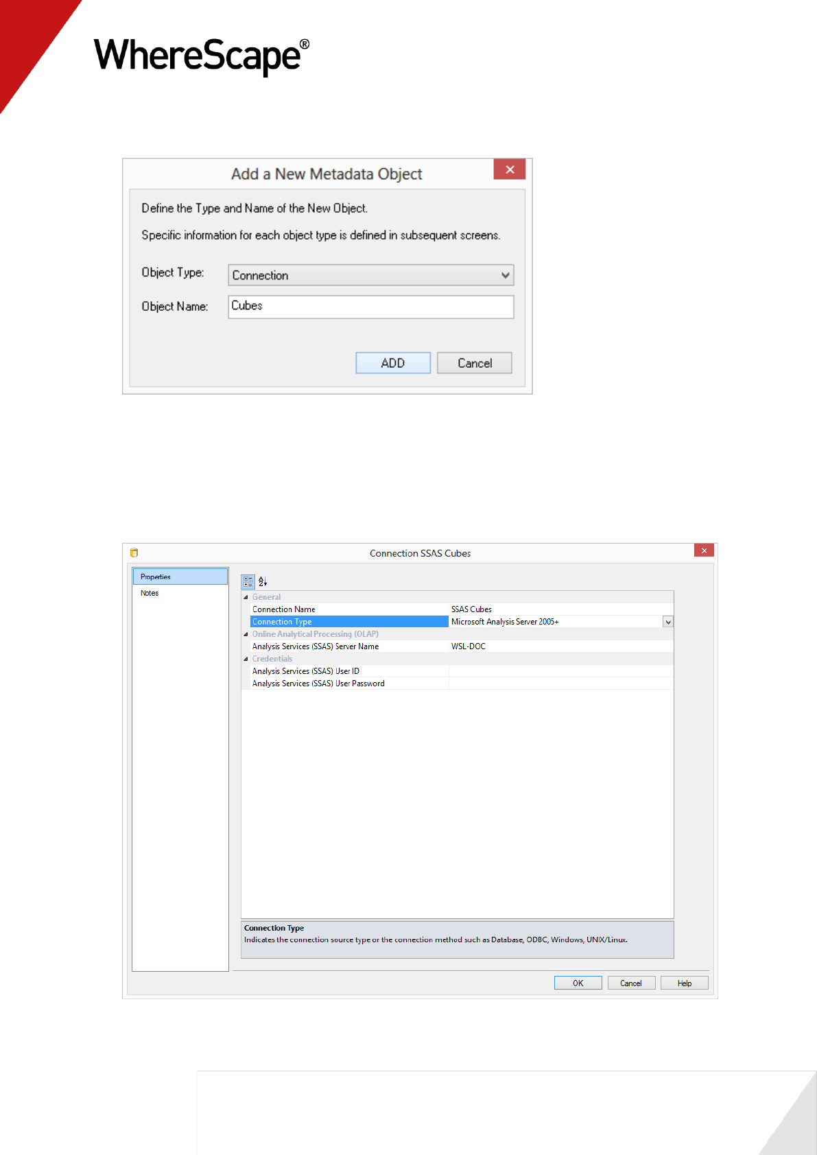
142
2 Enter a name of Cubes for the connection and click ADD.
3 The connection Properties screen displays. Select the connection type Microsoft Analysis
Server 2005+.
Enter the name of the server for the Analysis Server. Leave the username and password
blank.
Enter the server and database details for your Analysis Services server.
A sample is shown here. Click OK on the connection screen.

143
Note: Microsoft Analysis Services 2005 and 2008 use "Microsoft Analysis Server 2005+".
4 Expand the Connection object group in the left pane and double-click on the DataWarehouse
connection to bring up the Properties dialog.
5 The Properties dialog has some additional columns at the bottom of the screen. These are
required so that the data warehouse can be used as a source for the Analysis Services cubes.
These fields are:
OLAP Connection String
Connection Provider/Driver
Data Warehouse Server
Data Warehouse Database ID
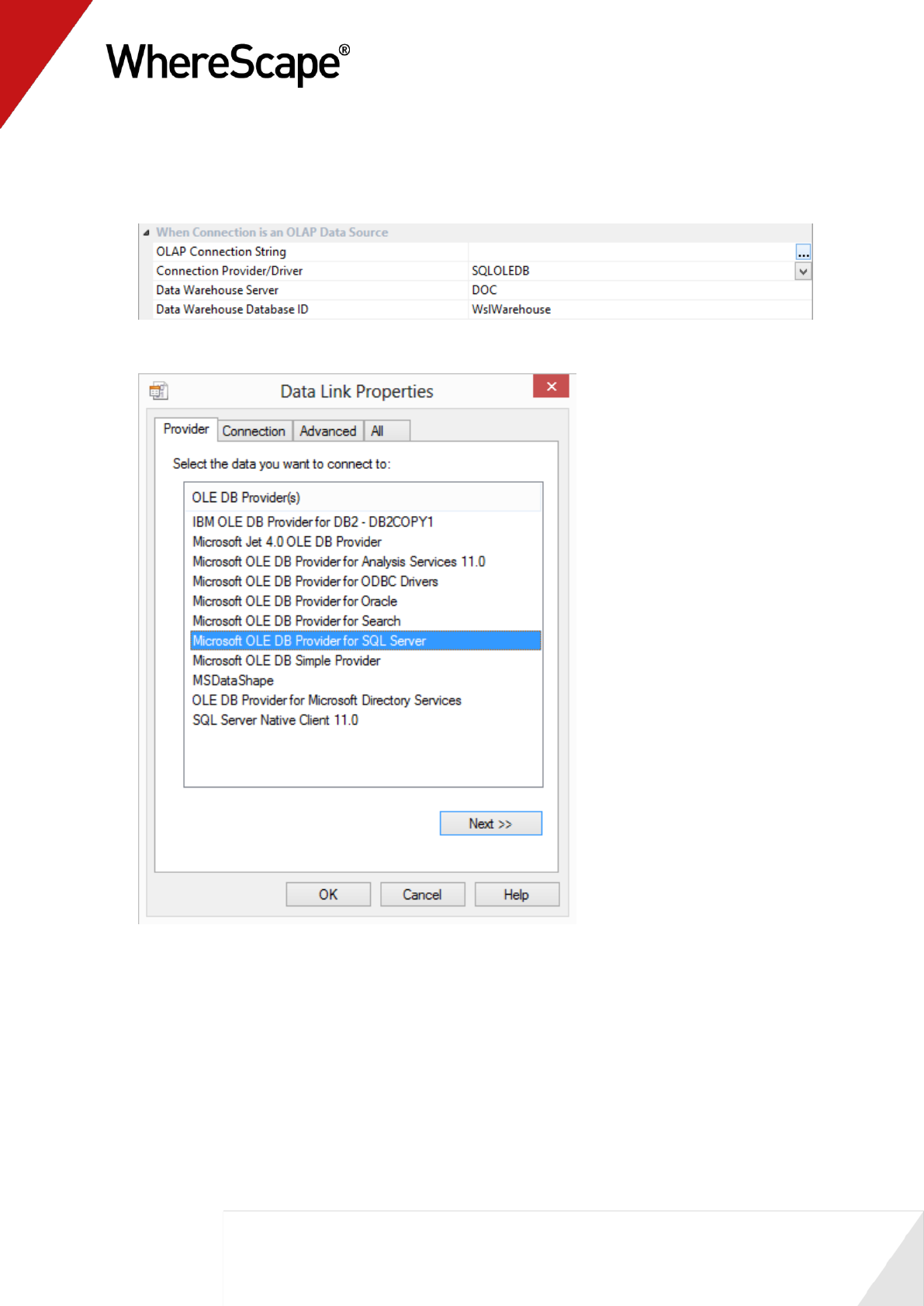
144
6 For a SQL Server data warehouse:
The OLAP Connection String is built using a wizard. To activate the wizard, click on the
eliipsis button.
7 On the Provider tab, select the OLE DB Provider and click Next.
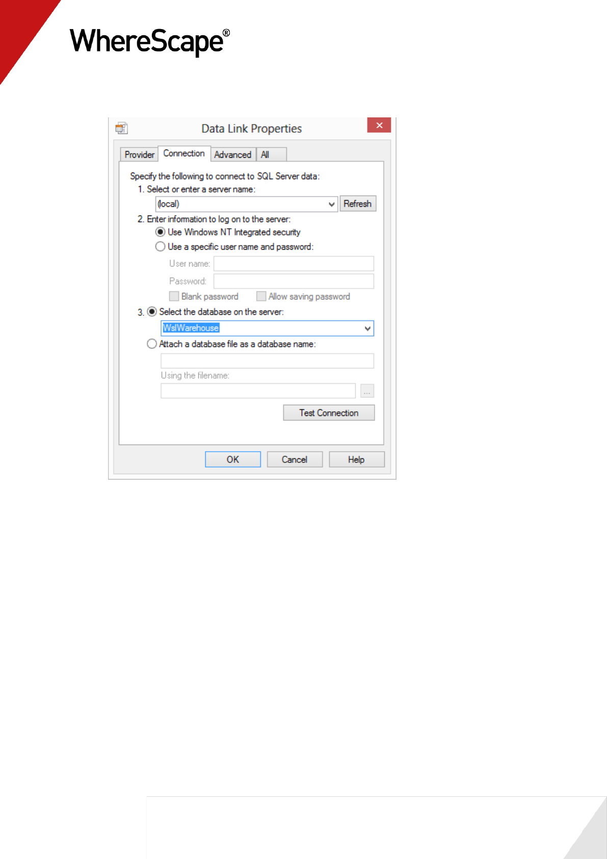
145
8 Enter the connection details and click Test Connection.
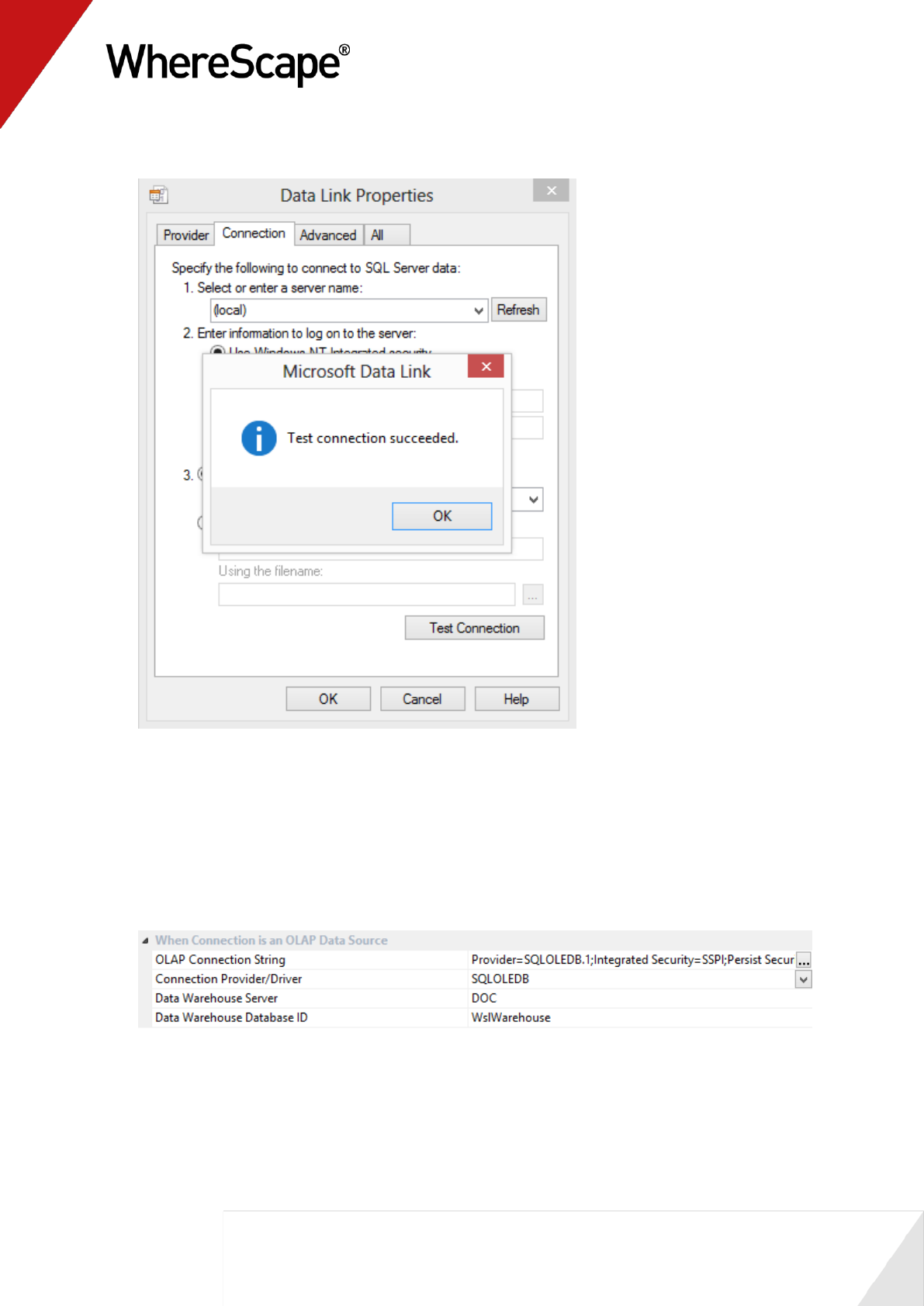
146
9 Click OK on the success message and then OK again on the Data Link Properties screen.
10 The OLAP connection string will be displayed on the connections screen.
11 Set the Connection Provider/Driver to SQLOLEDB
Set the Data Warehouse Server to the SQL Server server name
Set the Data Warehouse Database ID to the SQL Server database name
12 A SQL Server sample:
13 Click OK.
See Cube Connections for Other Databases (see "5.4 Cube Connections for Other Databases"
on page 184) for more details on Oracle and DB2.

147
14 Now you need to browse the DataWarehouse connection to see available fact tables.
Right-click DataWarehouse connection from the left pane and select Browse
Connection.
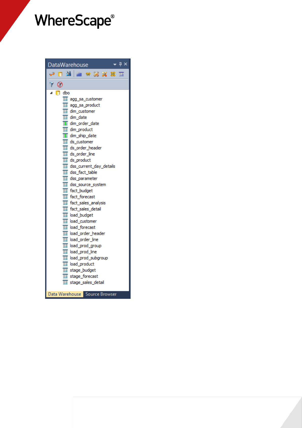
148
15 The following browse pane displays on the right.
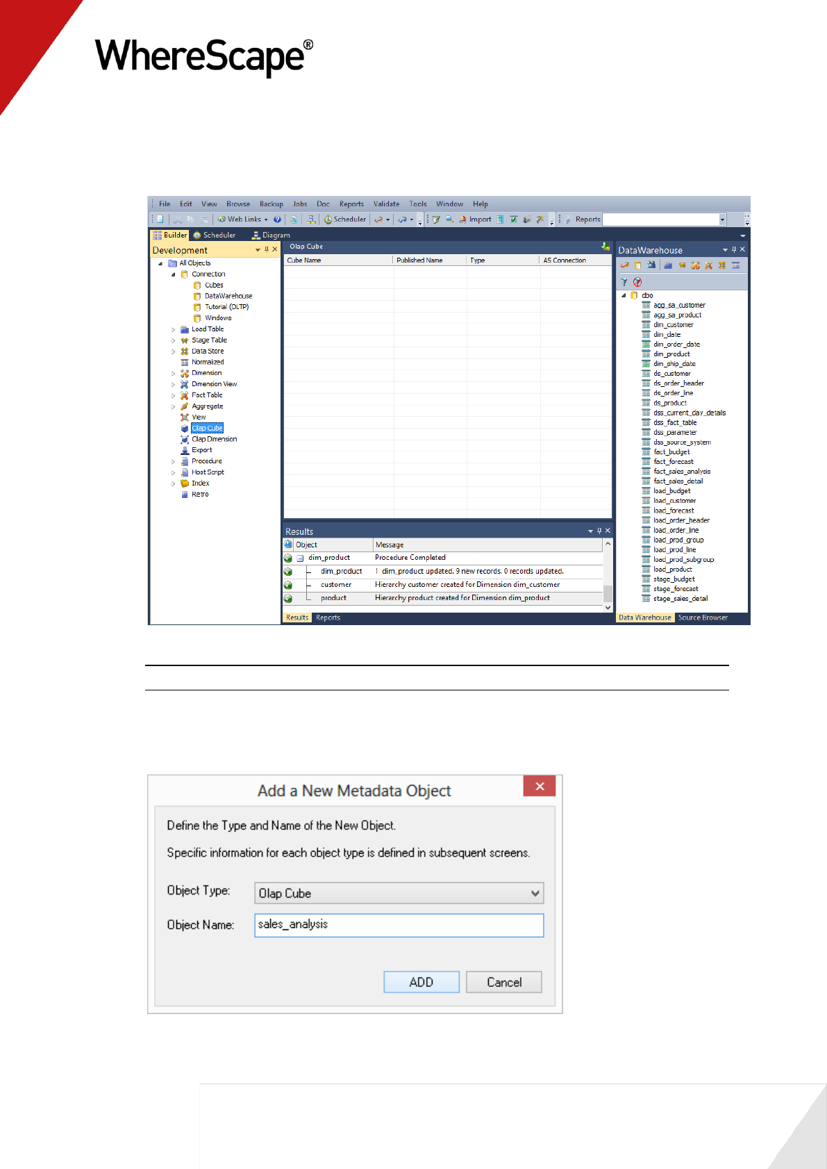
149
16 Double-click on the OLAP Cube object group in the left pane to list all cubes in the middle
pane. This makes the middle pane a drop target for cubes. Your screen should look something
like this:
Note: As OLAP Cubes have not been created yet, the middle pane is empty.
17 Drag fact_sales_detail from the browser (right pane) and drop it into the middle to create a
new OLAP Cube object. Give the OLAP Cube a name of sales_analysis as follows and click
ADD.
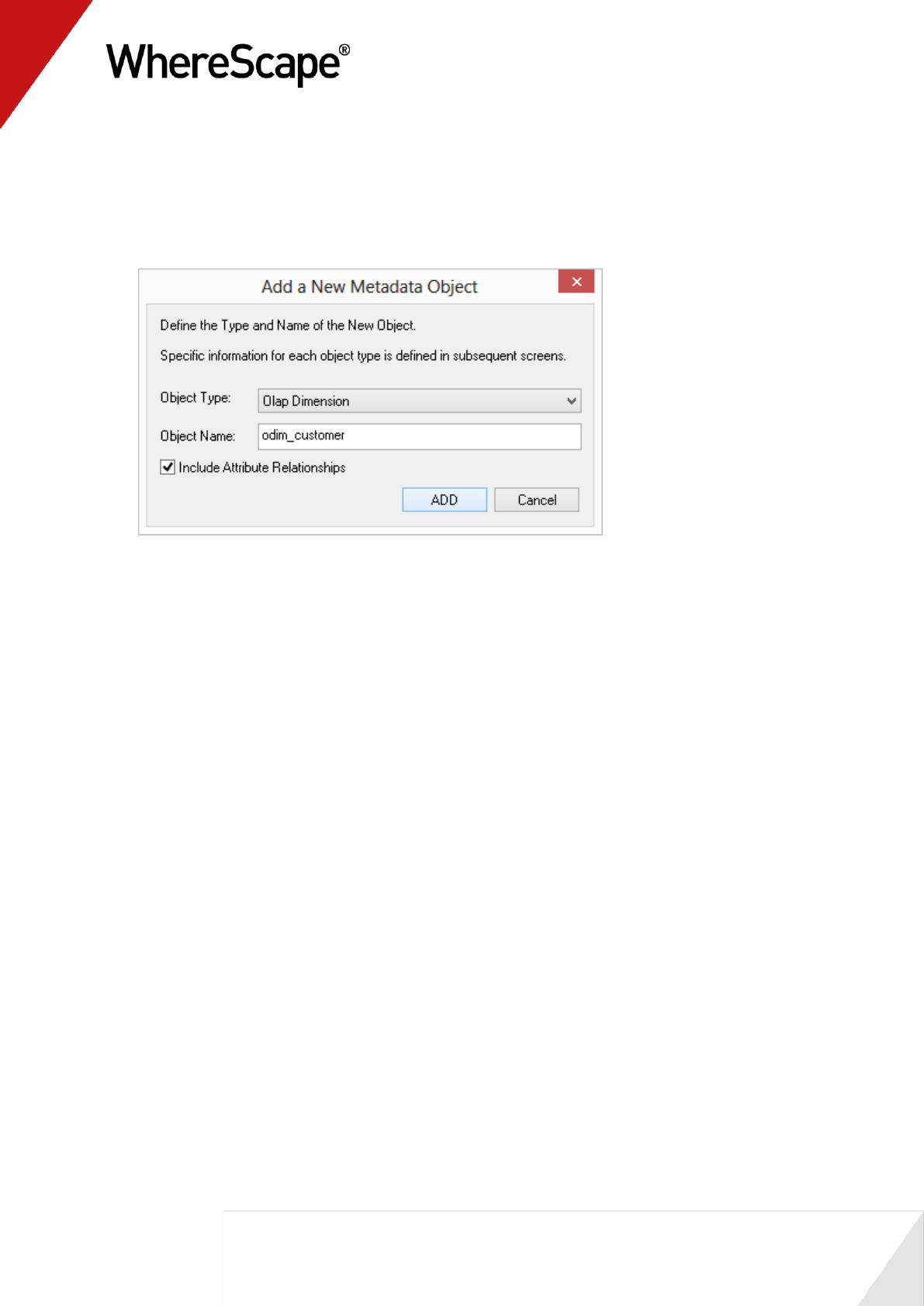
150
18 WhereScape RED will now cycle through each dimension associated with that fact table and
will create an OLAP Dimension object for each, displaying the following dialog first.
Tick the Include Attribute relationships check- box to include Attribute Relationships
in Analysis Services for this dimension.
Click ADD for the Customer dimension.
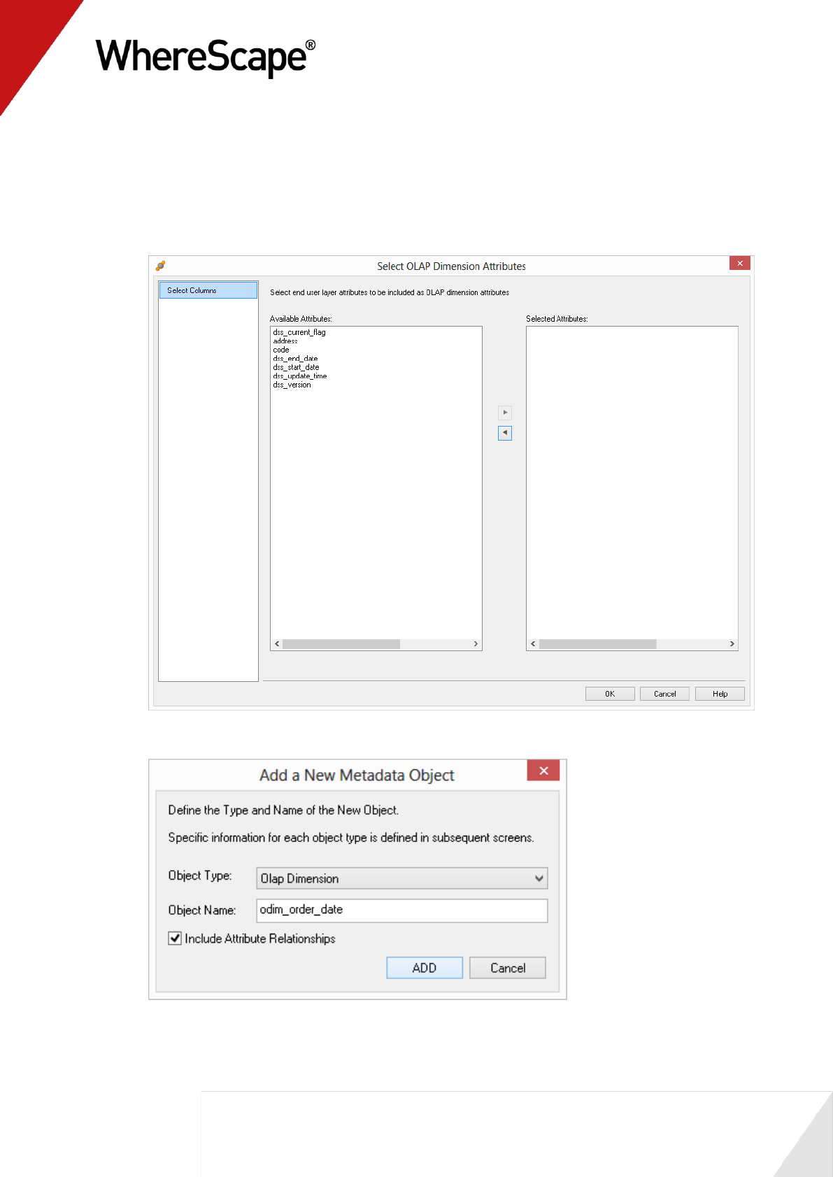
151
19 The following dialog appears, prompting you to select the attributes to be included in the
Customer OLAP dimension. The attributes available for selection are in the left column. To
select an attribute, click on the attribute in the left column and click >. This will move the
attribute to the right column.
To de-select an attribute, click on the attribute in the right column and click <. This will
move the attribute to the left column.
20 Repeat steps (9) and (10) for the remaining OLAP Dimensions.
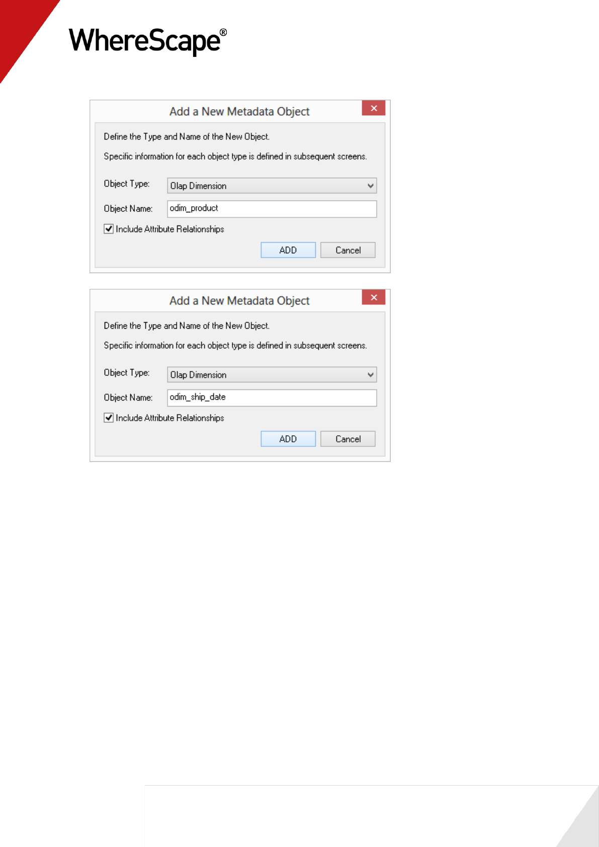
152
21 The Manage cube measures dialog is displayed next. Remove all non-measure columns (that
is, columns that cannot be aggregated) from the Measure list by highlighting them and
clicking the Remove button.
The columns to remove are:
order number
order line no
product code
customer code
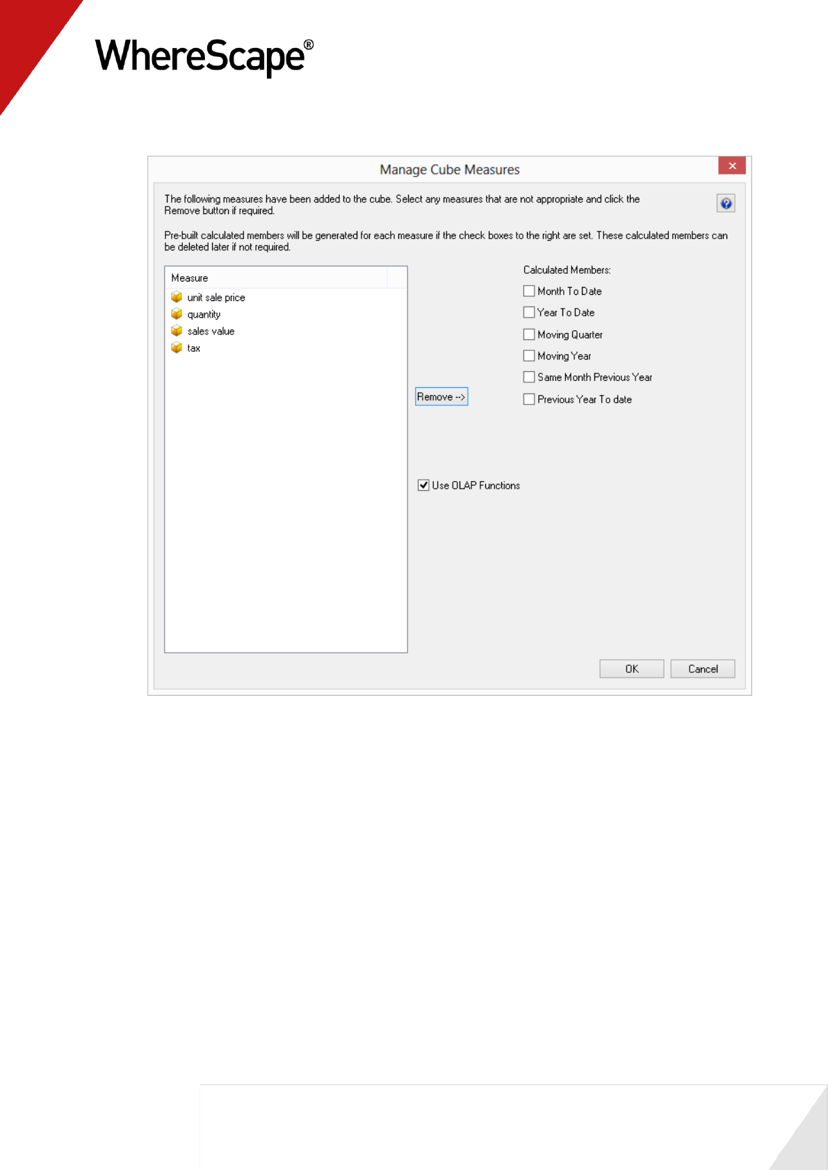
153
22 At this stage, your dialog should look like this:
23 Choose to create some date based calculated members using OLAP functions by selecting the
Month to date, Year to date, and Use OLAP functions check-boxes.
The calculated measures drop-downs display below.
24 Select the required date hierarchy information. Specifically:
for Date Dimension, select dim_order_date and the Date Hierarchy will automatically
be populated with calendar
for Month Level, select order cal month
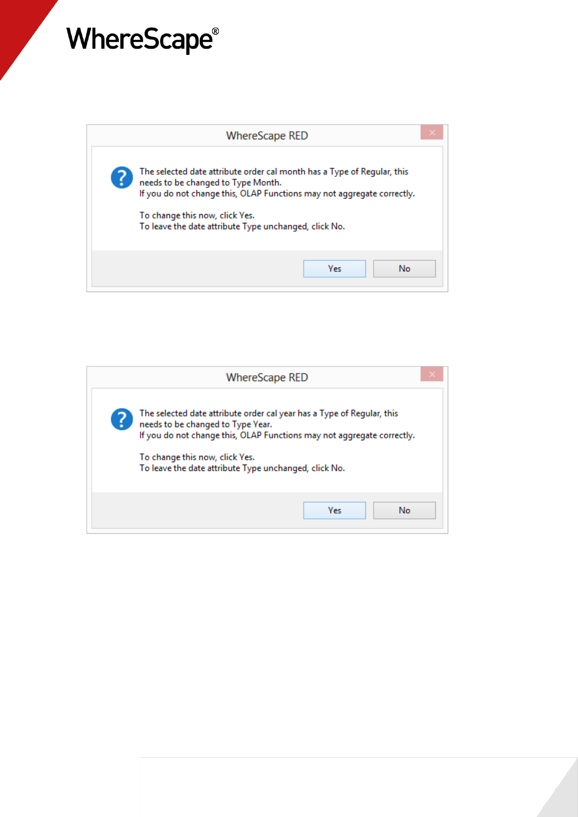
154
25 After selecting the Month level, you will be asked to confirm changing the attribute type to
Months for the the order cal month attribute in Analysis Services as follows. Click Yes.
26 For Year Level, select order cal year.
Similarly, selecting the Year level, you will be asked to confirm changing the attribute
type to Years for the the order cal year attribute in Analysis Services as follows. Again
click Yes.
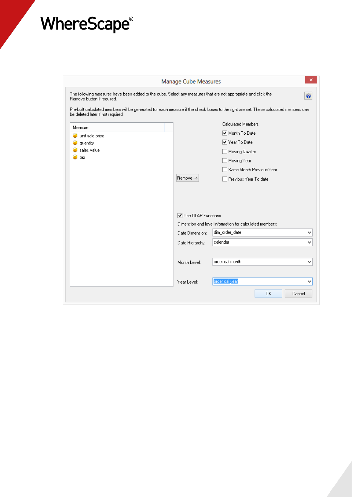
155
27 Your Manage cube measures dialog should now look like this. Click OK to complete the
definition of the cube.
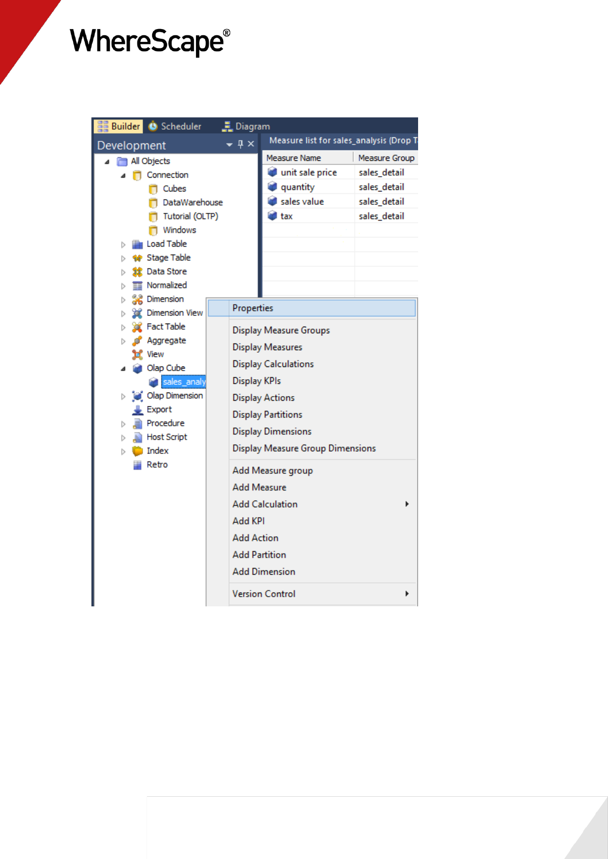
156
28 Right-click on the OLAP Cube sales_analysis in the left pane and select Properties.
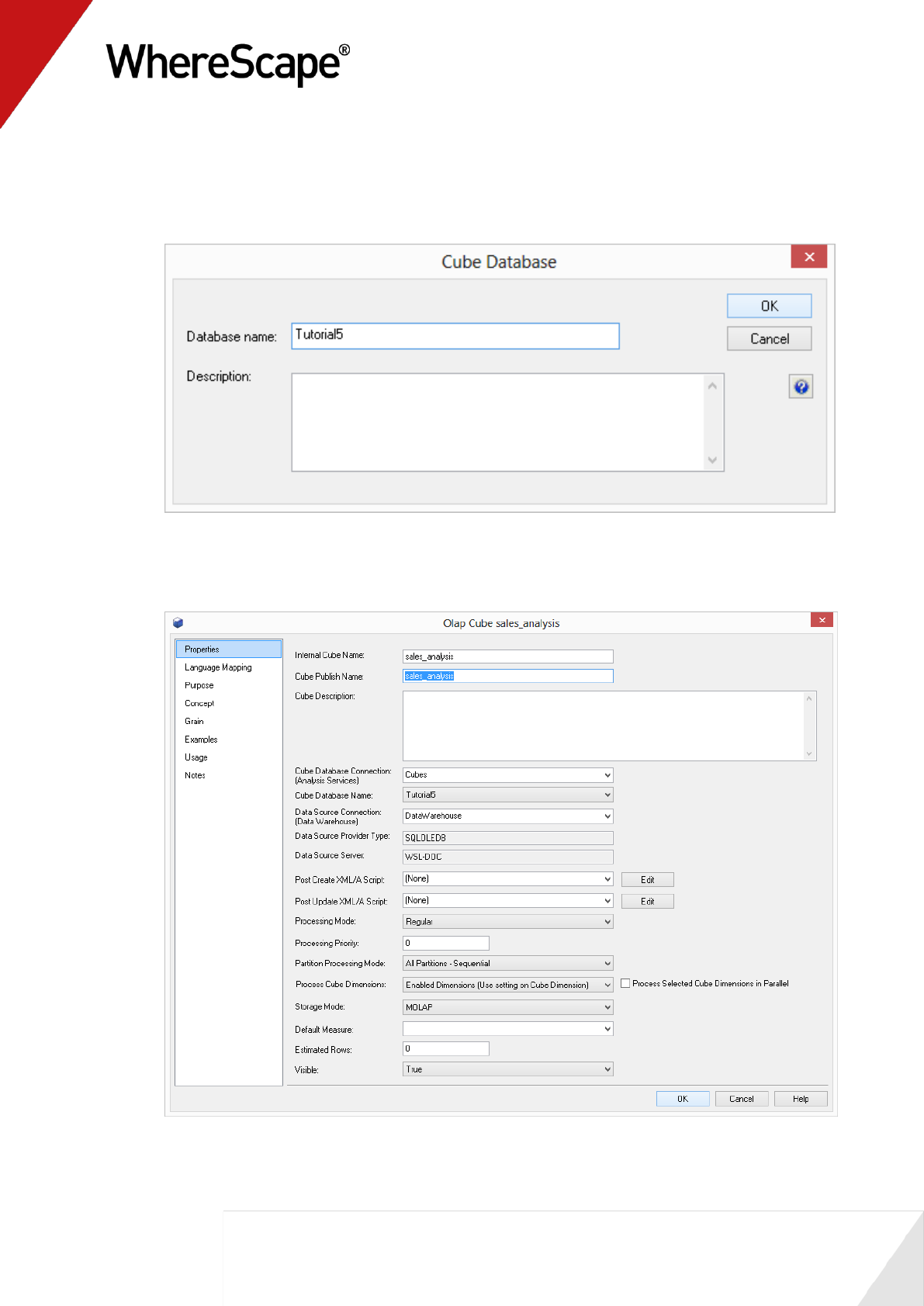
157
29 Click on the drop-down list for the Cube Database name field and select the option (Define
New Cube Database).
30 This will bring up the Cube database dialog box. Enter a new cube Database name of
Tutorial5. Click OK.
31 Change the Cube publish name to be sales_analysis and ensure the Cube database
connection is Cubes and the Cube Database Name is Tutorial5.
Click OK to close the dialog and save the changes you've made.
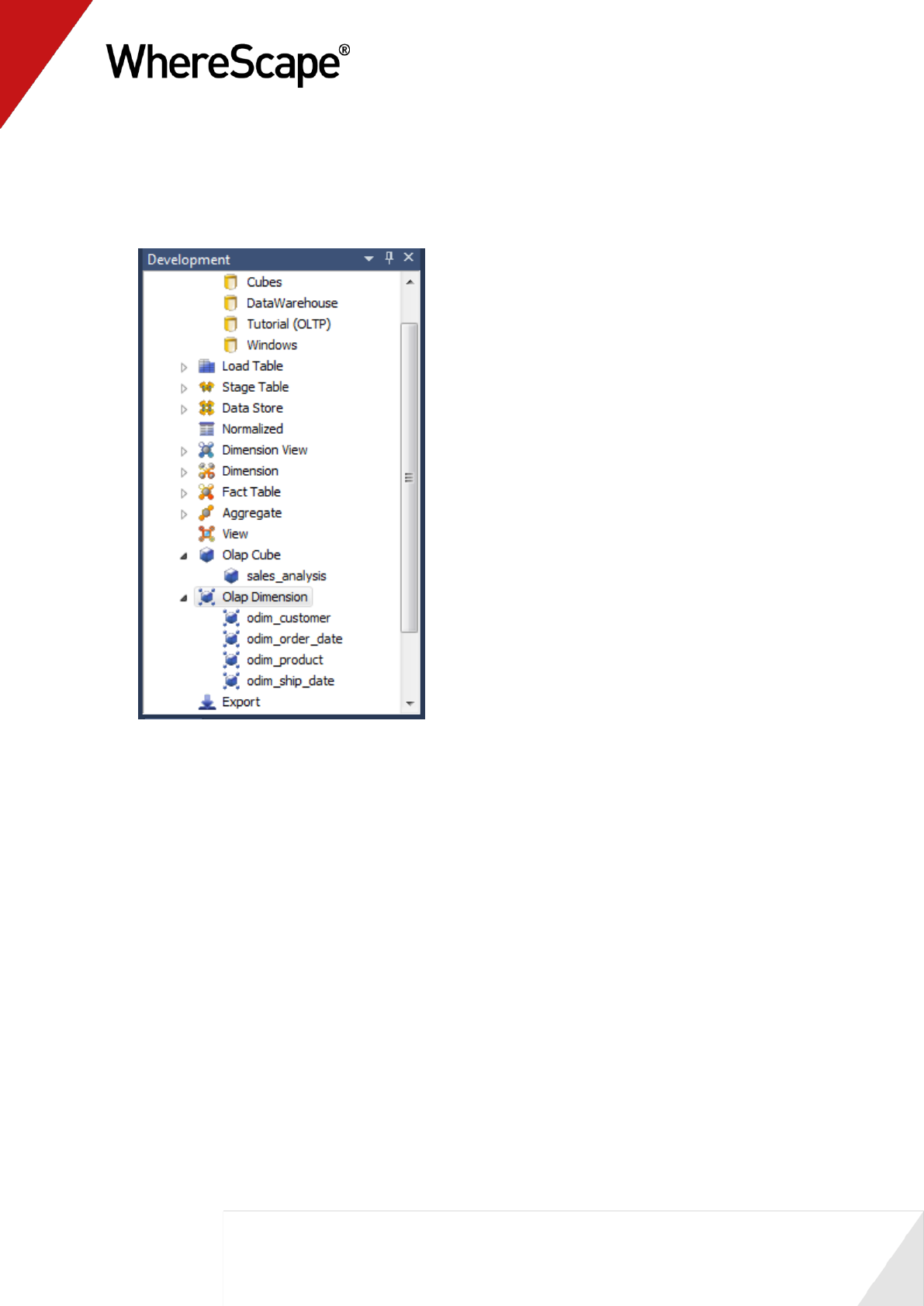
158
32 Now you need to check that the date dimension supports using OLAP functions.
Expand the OLAP Dimension object type in the left pane to display the four OLAP
Dimensions.
Your object tree should contain the following OLAP Dimensions.
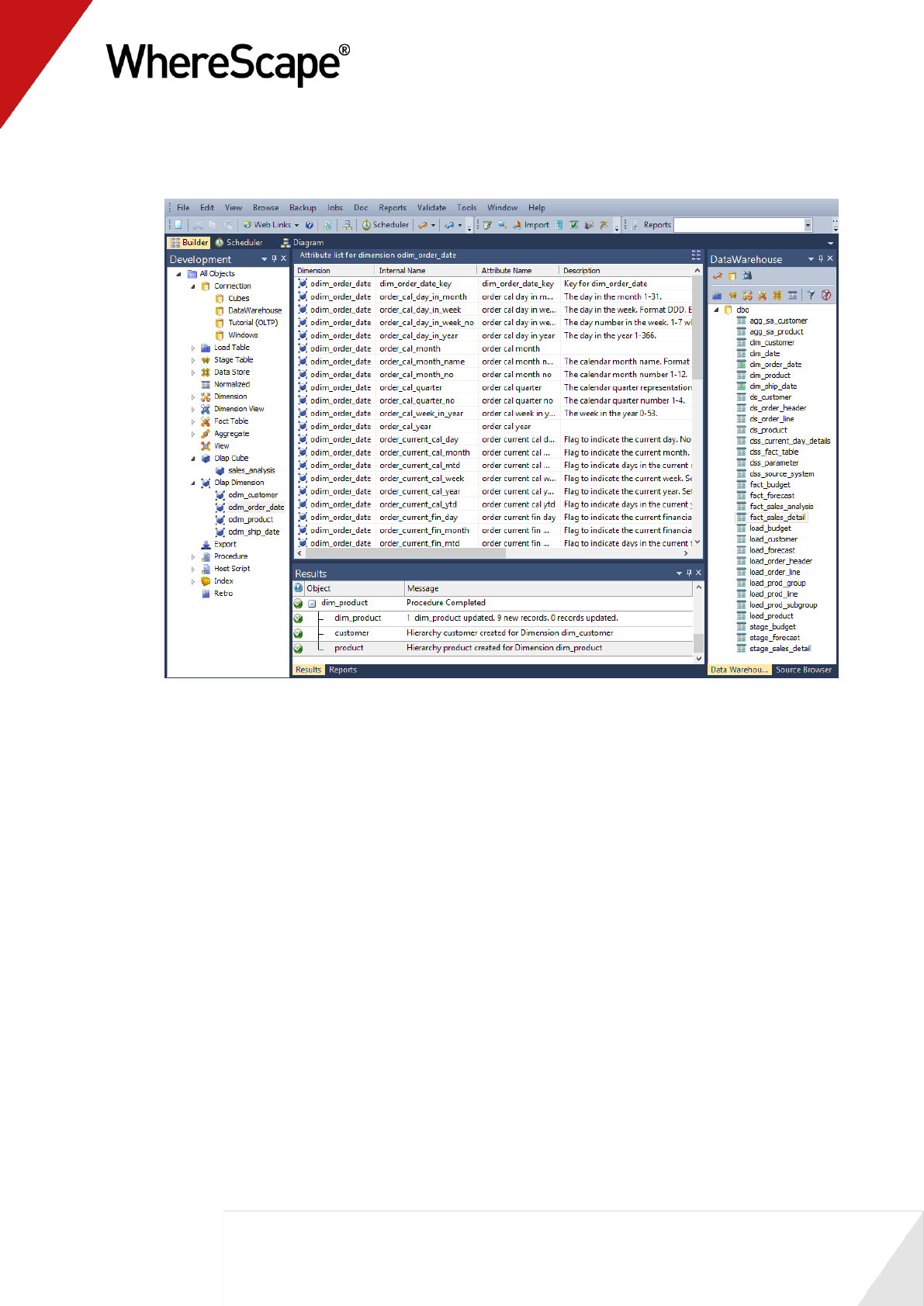
159
33 Click on the odim_order_date OLAP Dimension in the left pane to show the dimension
attributes in the middle pane as below.
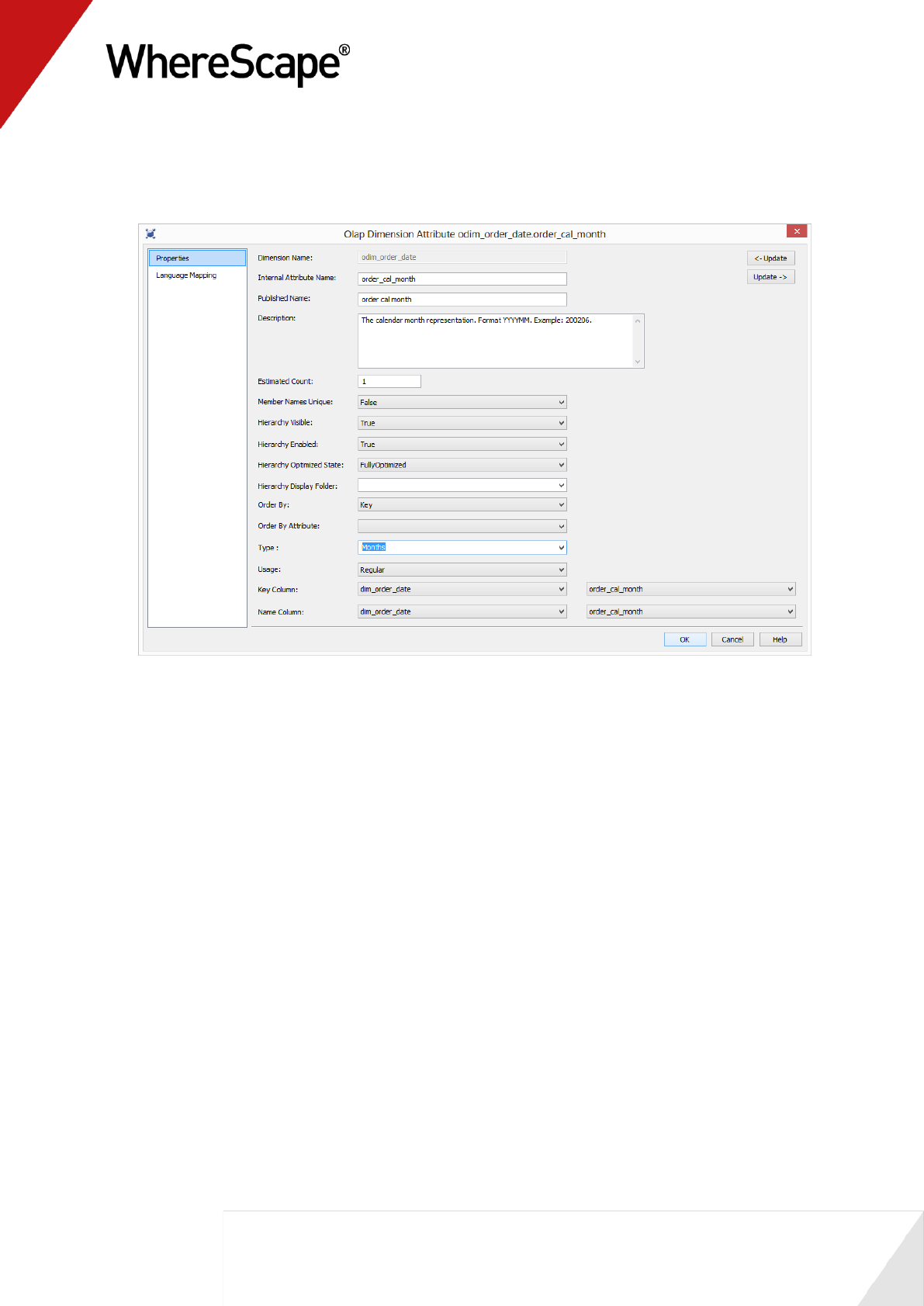
160
34 Right-click on the order_cal_month attribute and select Properties.
This displays the Attribute Properties dialog. Check the Type is set to Months. If not,
change it. Click OK.
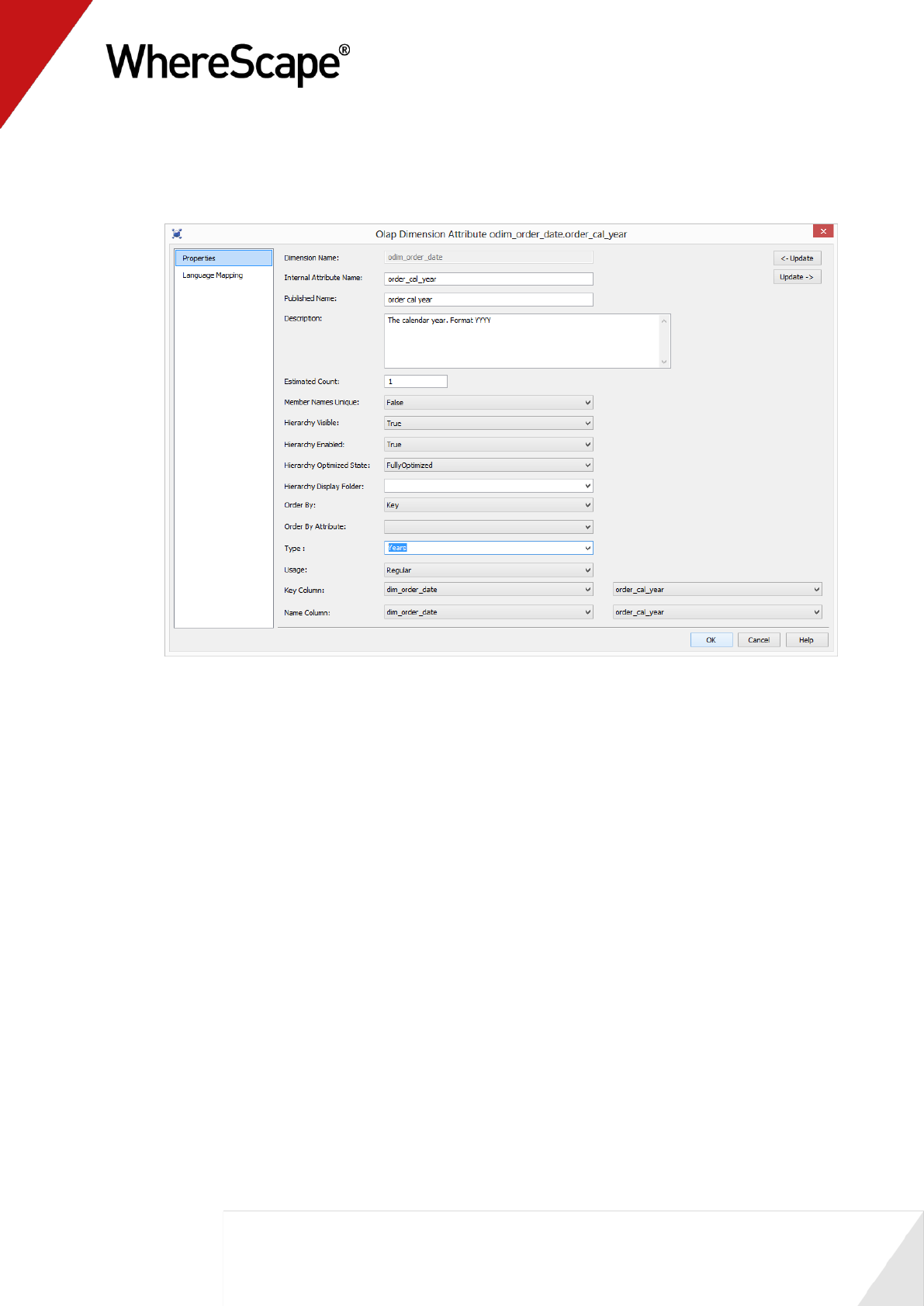
161
35 Repeat the process for the order_cal_year attribute, checking the Type is set to the Years
and changing it if it is not.
Click OK.
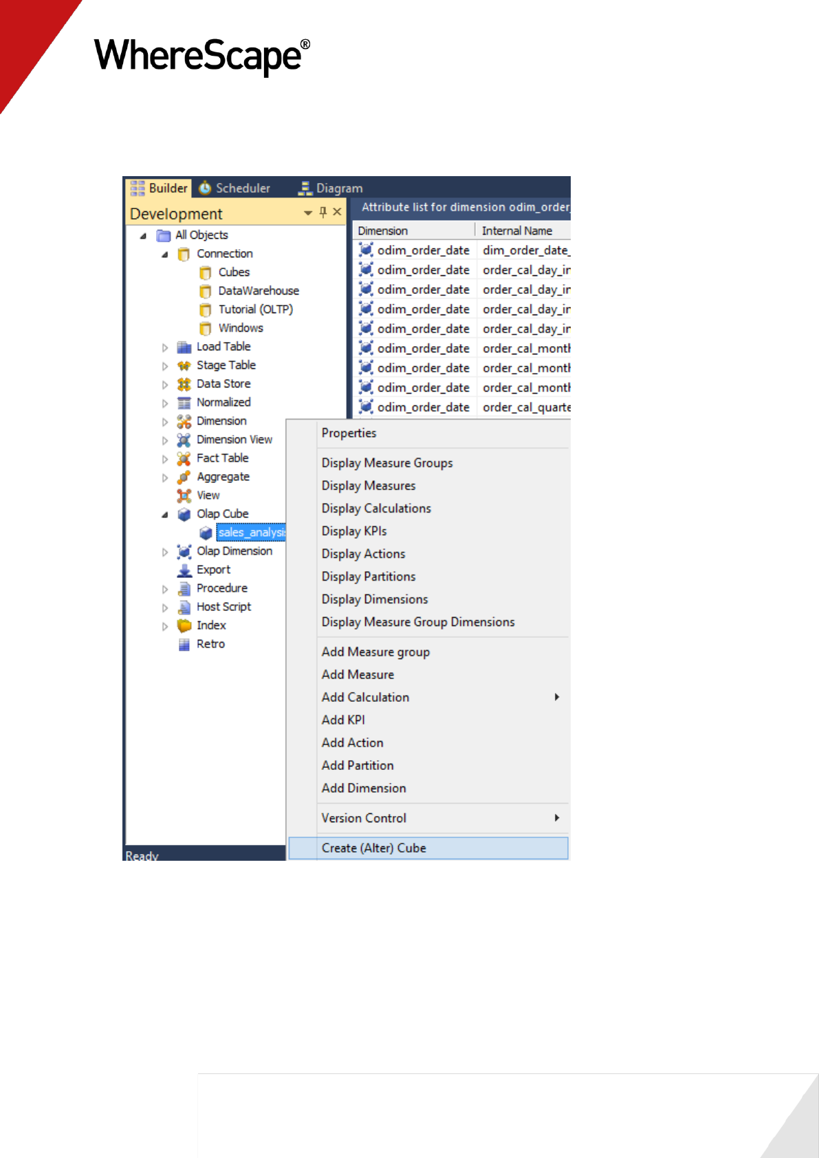
162
36 To create the cube in Analysis Services, right-click on the sales_analysis olap cube in the left
pane and select Create (Alter) Cube.

163
37 This will open the WSL Cube executable that connects to Analysis Services to create the
sales_analysis cube structure.
You will see the successful completion in the results pane.
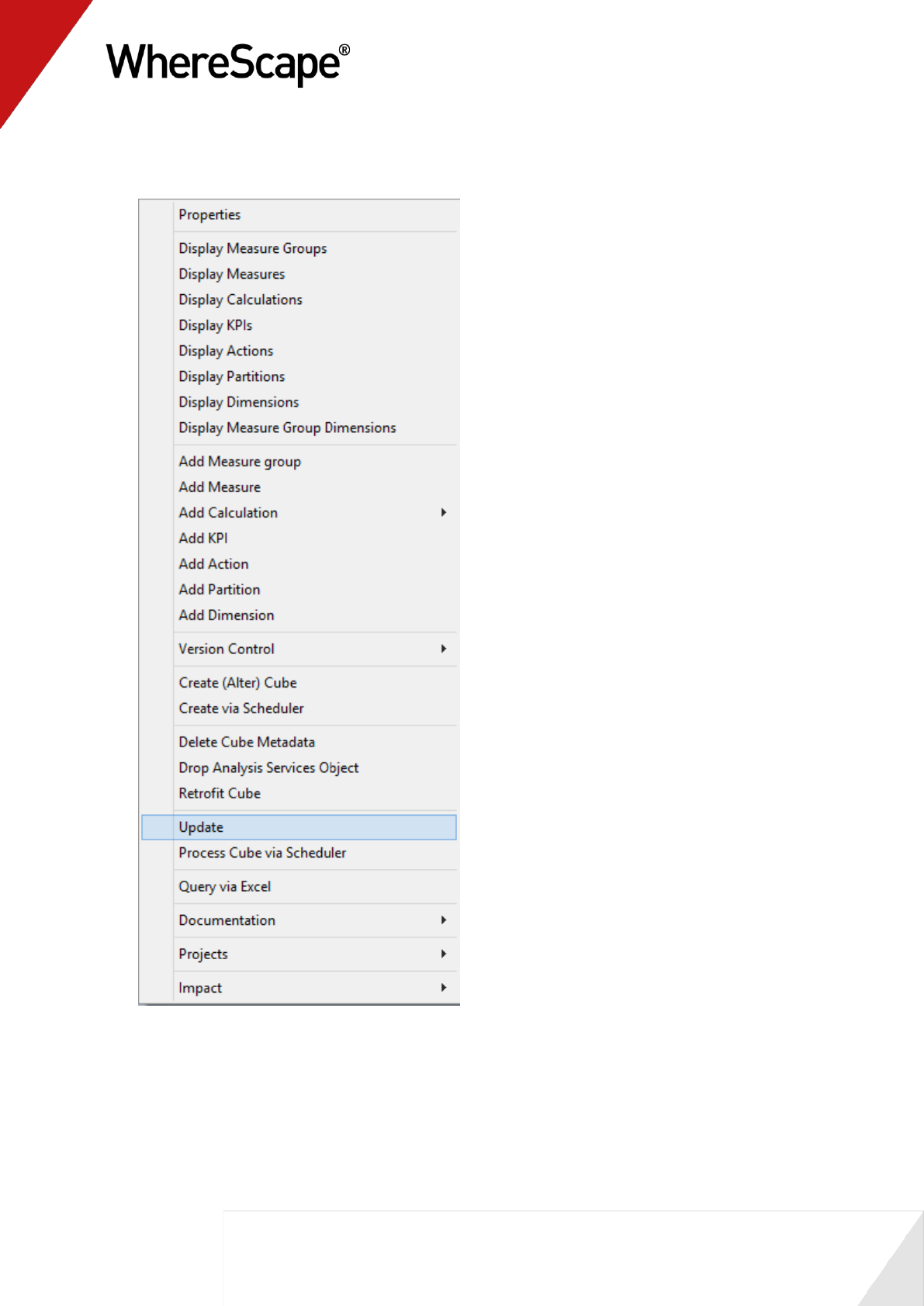
164
38 To process the cube sales_analysis in Analysis Services right-click the sales_analysis cube in
the left pane and select Update.
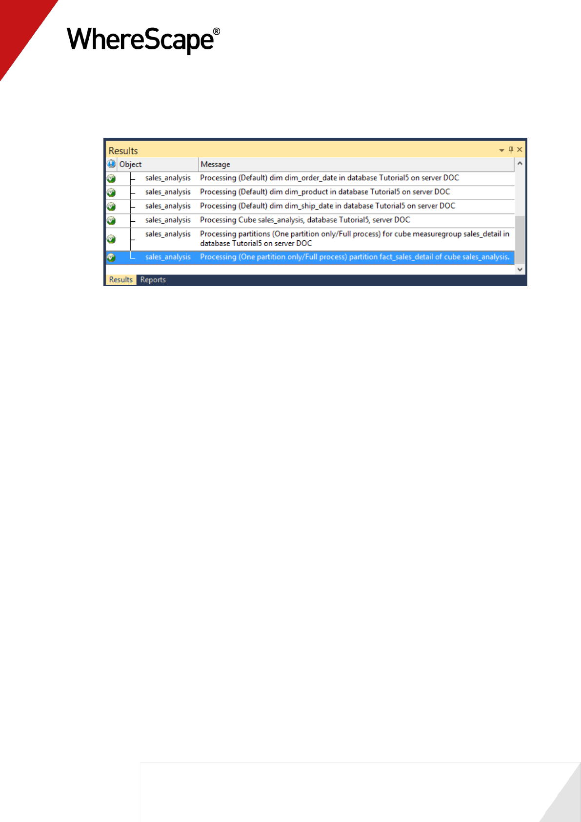
165
39 This will open the WSL Cube executable to process data into the cube structure. Once the
cube is processed it can be viewed. Again, you will see the successful completion in the
results pane.
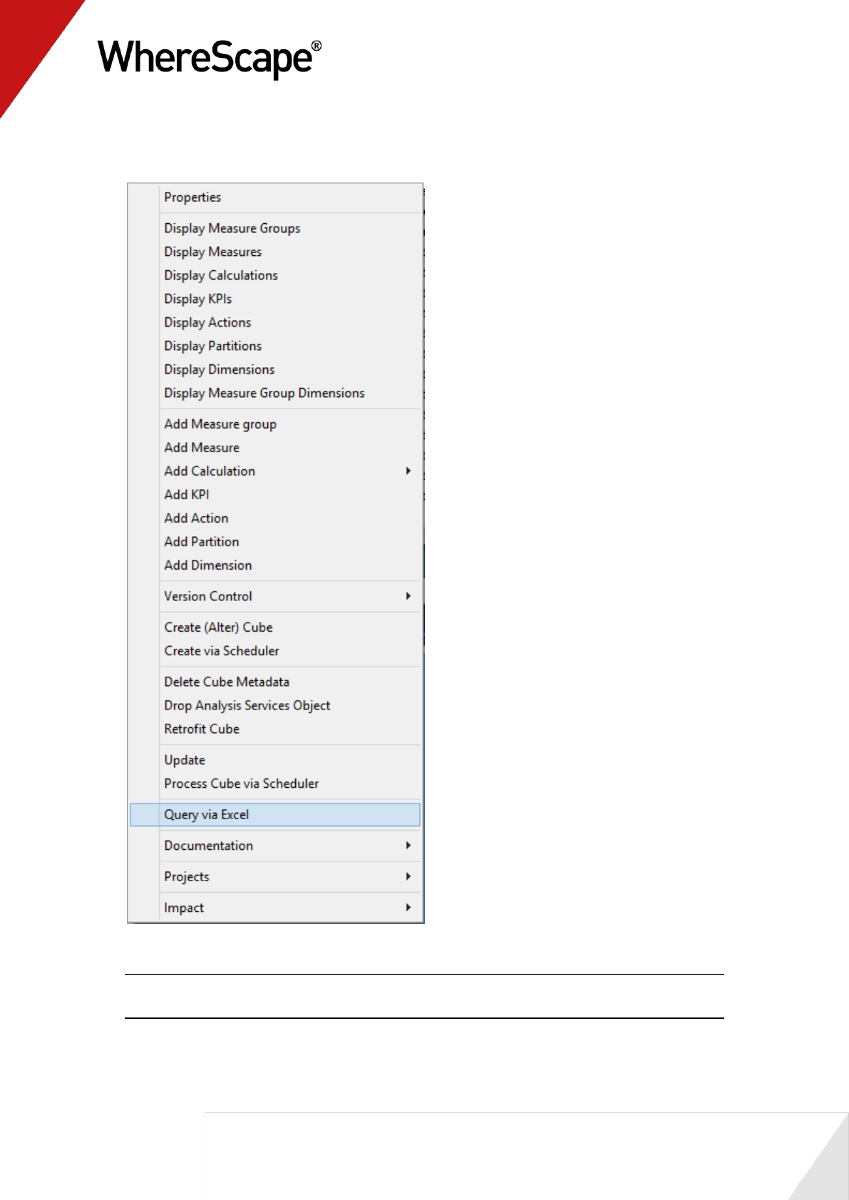
166
40 To view the cube in Excel right-click the sales_analysis cube in the left pane and select
Query cube Via Excel as follows.
41 This will open Excel if it is installed.
Note: If Excel displays a security notice dialog box, click Enable.
However, note that this dialog box may not be displayed.
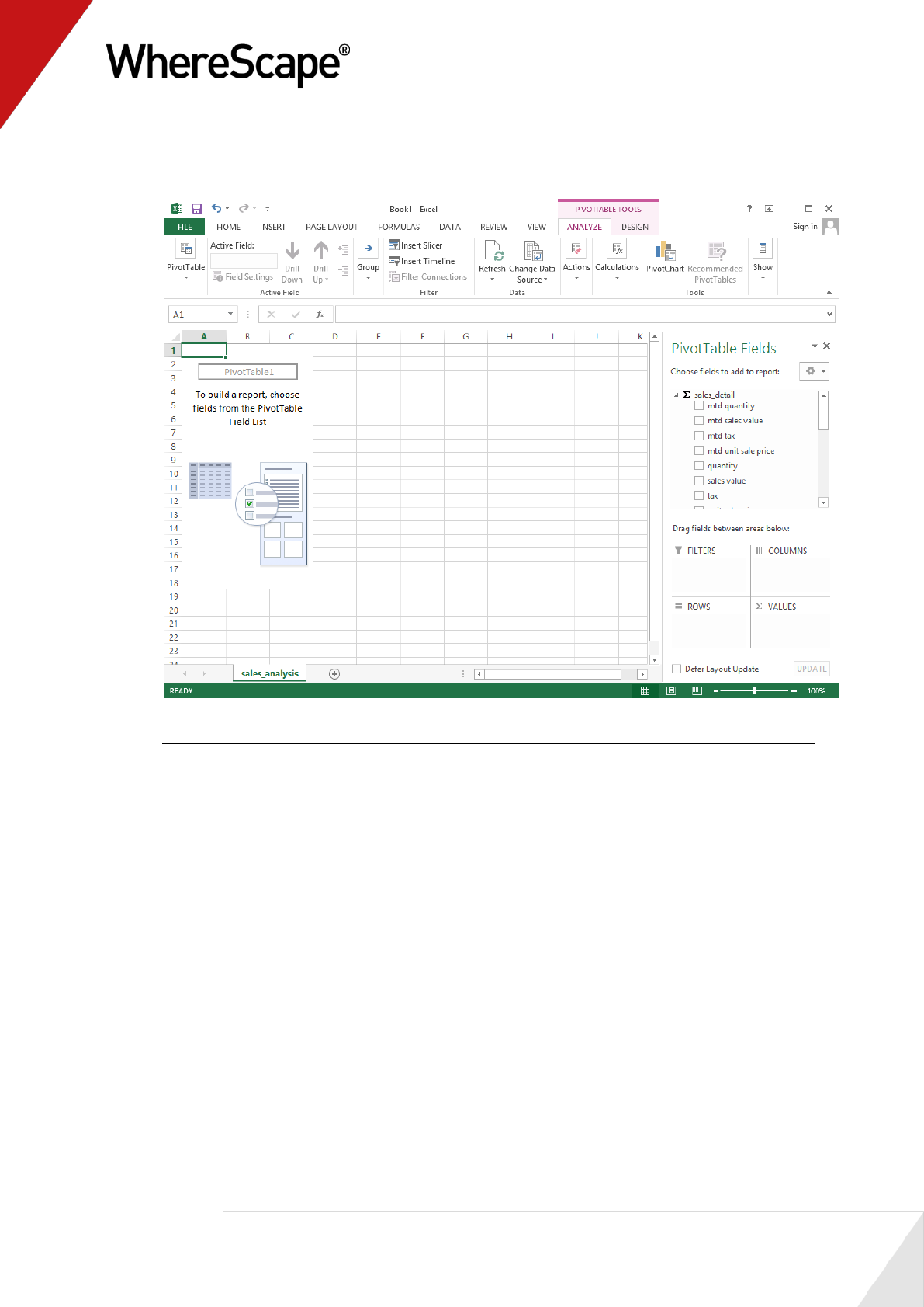
167
42 Excel then opens a connection to the cube for querying in a pivot table:
Note: In order for Excel to open the cube the OQY file extension in Windows explorer needs
to be associated with Excel.
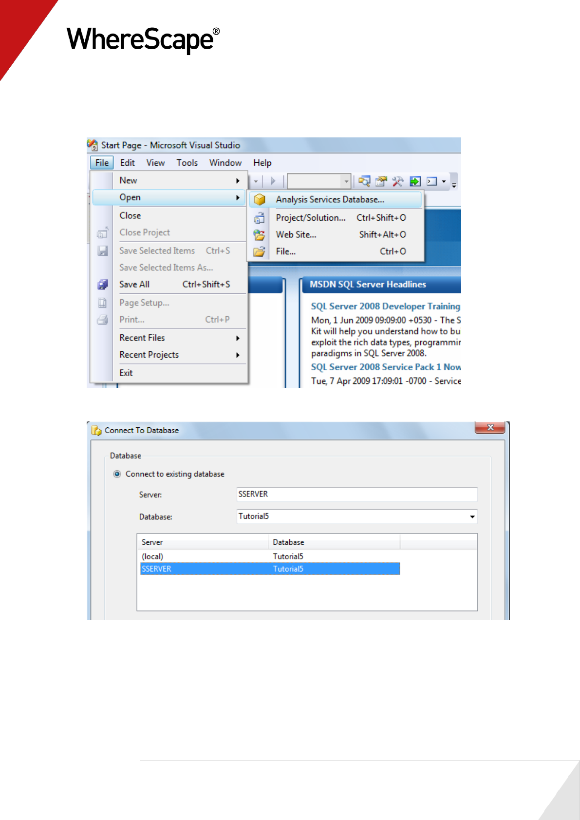
168
43 In addition, the cube structure can be opened in the Microsoft Business Intelligence
Development Studio (BIDS). Open BIDS in Windows, then select Open / Analysis Services
Database.
44 Choose the server and Tutorial5 cube database. A sample is shown. Click OK.
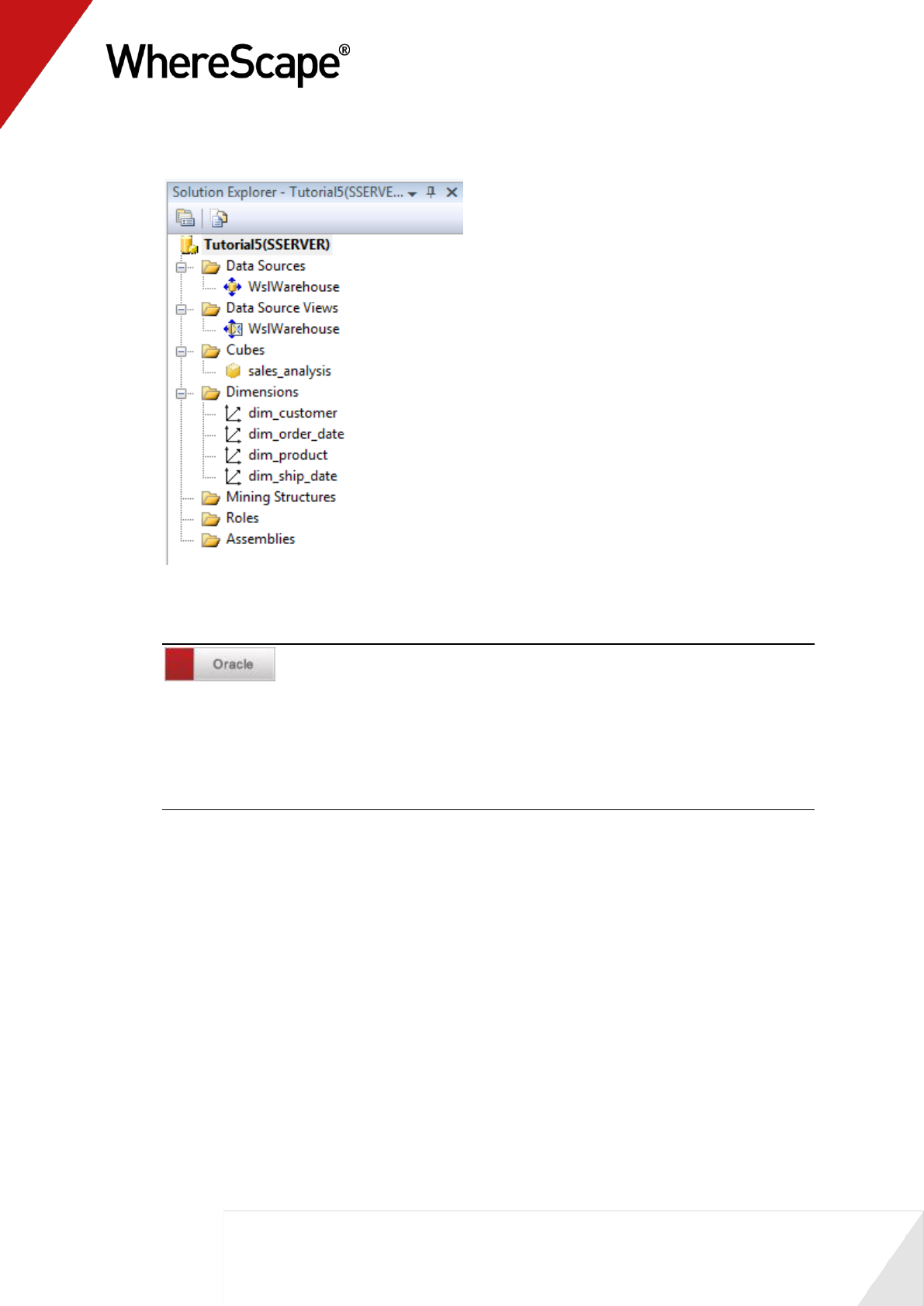
169
45 This now displays the cube database definition from the Analysis Services server.
46 Close BIDS when finished.
In the latest version of RED, the default 0 key date for all databases has been
set to 1st Jan 1753. Prior to 6.5.4.2 however, procedure update_dim_date uses sysdate-700000
which gives a date in year 0095. SSAS does not support dates before year 0100 using the
oracle OLEDB driver. If using a previous version of RED, or upgrading from a previous
version, it will therefore be necessary for you to replace 'sysdate - 700000' with
'TO_DATE('17530101','YYYYMMDD')' in procedure update_dim_date and to recreate the
dim_date table.
You are now ready to proceed to the next section - Adding a Measure Group (see "5.3 Adding
a Measure Group" on page 170)
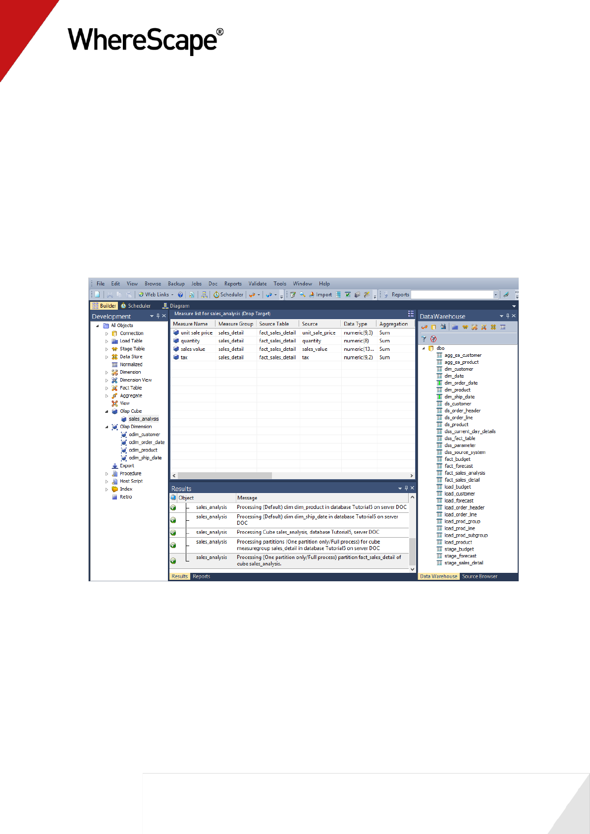
170
5.3 Adding a Measure Group
A cube can contain multiple Measure Groups. In WhereScape RED, a Measure Group relates to a
relational star schema.
The cube ties Measure Groups together through shared dimensions that are conformed in the
relational data warehouse.
Measure Groups can be added to an existing cube by dragging additional fact tables into the cube.
1 Click on the OLAP Cube sales_analysis in the left pane to show the Measures associated with
the cube.
Your screen should look something like this:
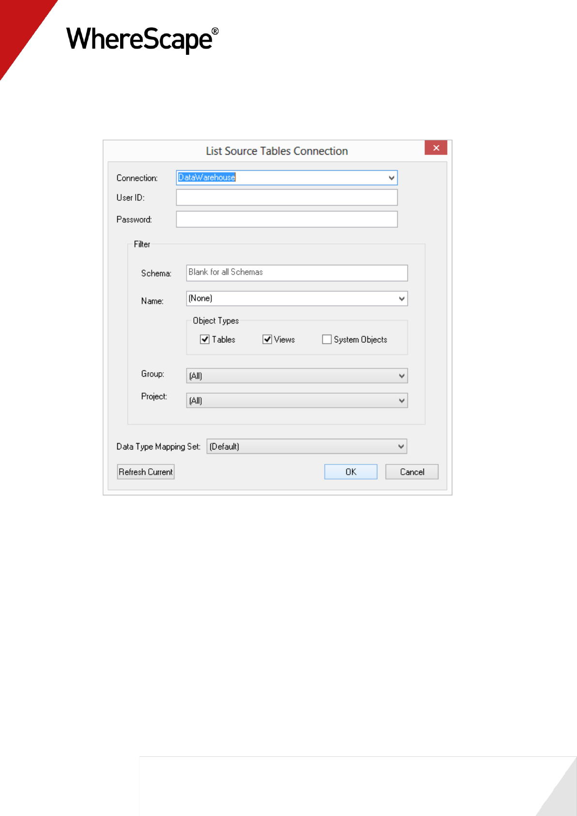
171
2 Now you need to browse the DataWarehouse connection to see available fact tables.
Right-click DataWarehouse connection from the left pane and select Browse
Connection.
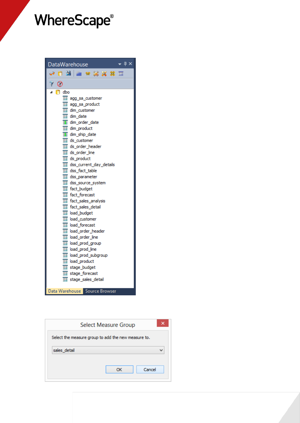
172
3 The following browse pane displays on the right.
4 Drag the fact_budget table into the middle pane. The following dialog will appear. Select
Cancel.
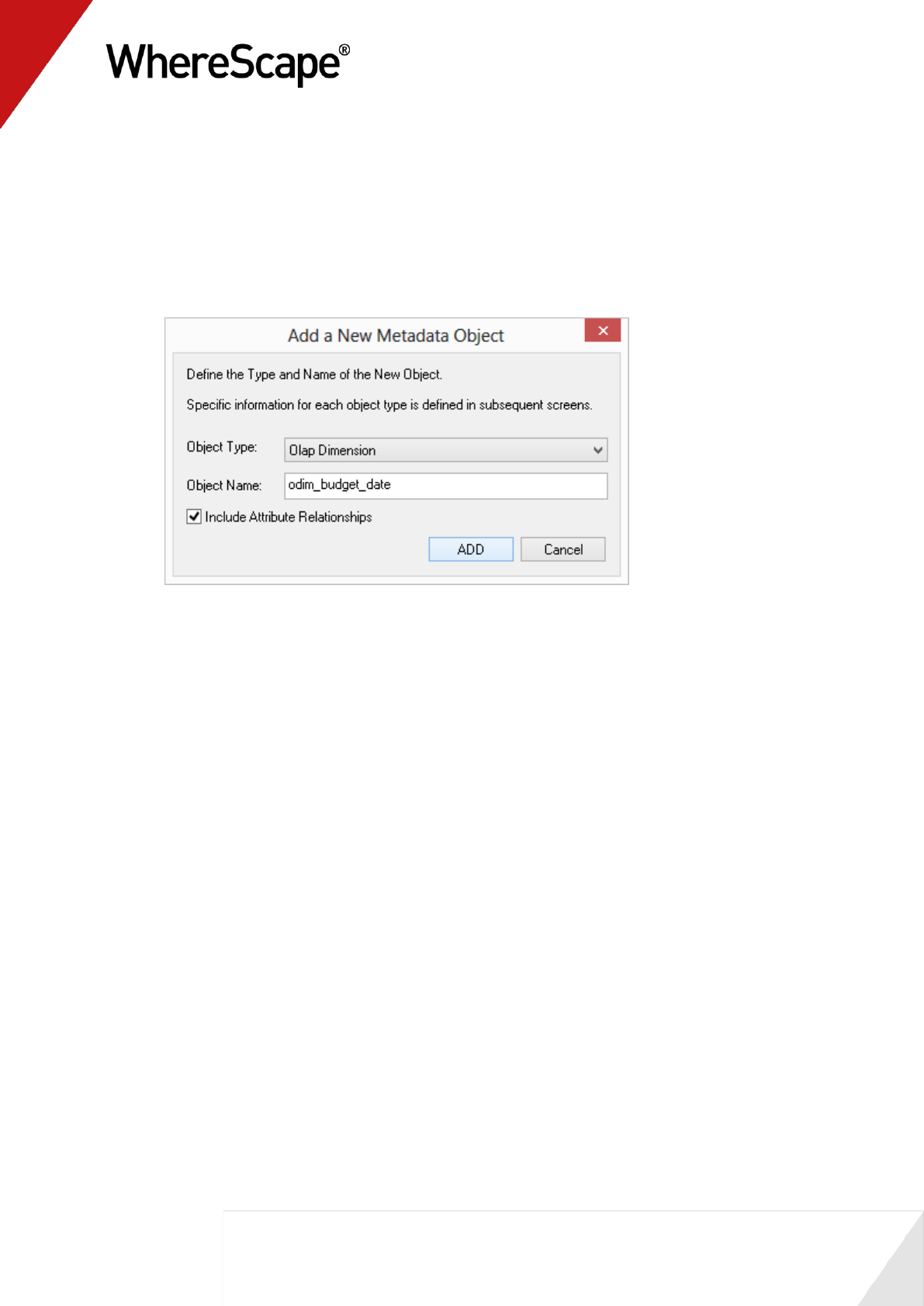
173
5 WhereScape RED will confirm that it is OK to add a new OLAP Dimension for the date
dimension.
Change the Name of object to odim_budget_date.
If you want to include Attribute Relationships in Analysis Services for this dimension, tick
the Include Attribute Relationships check-box.
Click ADD.
6 Click OK on the Attributes screen.
7 The Manage Cube Measures dialog displays.
Remove all non-measure columns (that is, columns that cannot be aggregated) from the
Measure list by highlighting them and clicking the Remove button. The columns to remove
are:
Product Code
Customer Code
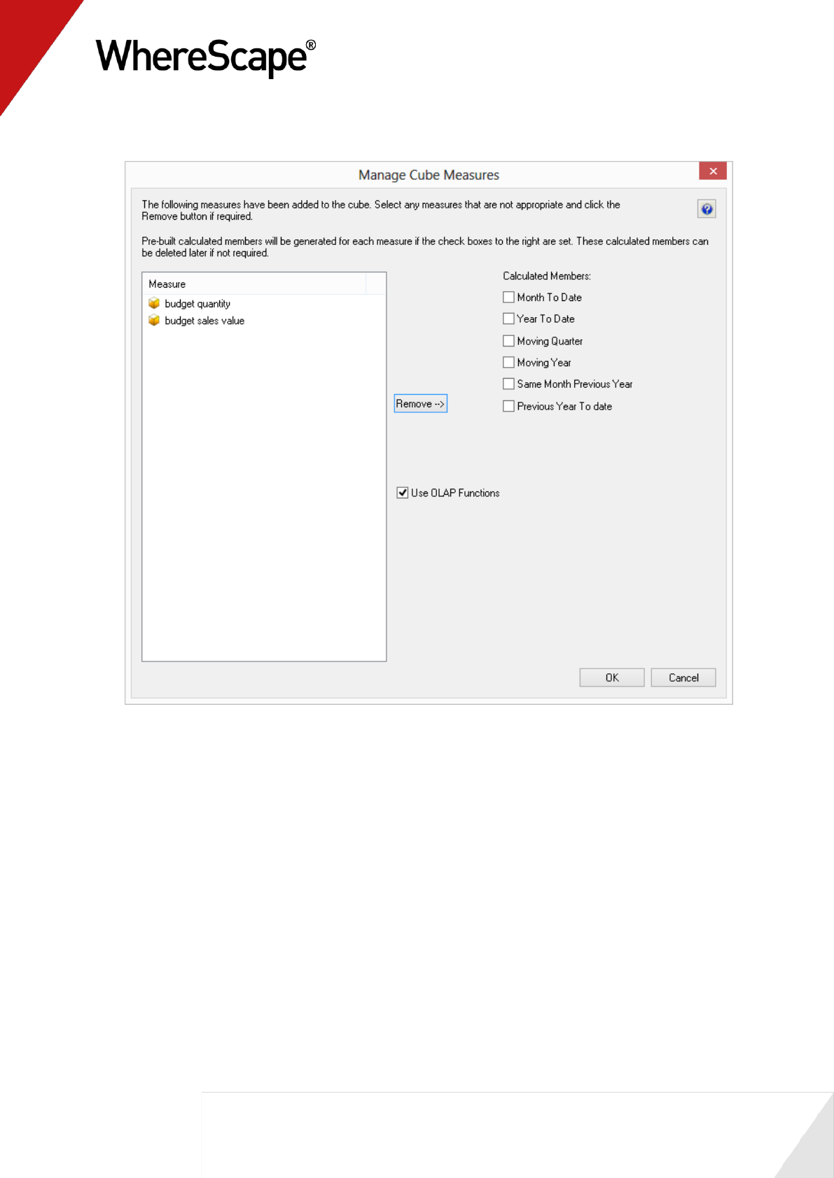
174
8 At this stage, your dialog should look like this.
9 Choose to create some date based calculated members using OLAP functions by selecting the
Month to date, Year to date, and the Use OLAP Functions check-boxes.
The calculated measures drop-down list display below.
10 Select the required date hierarchy information. Specifically:
for Date Dimension, select Date Dimension and the Date Hierarchy will automatically
be populated with calendar
for Month Level, select cal month
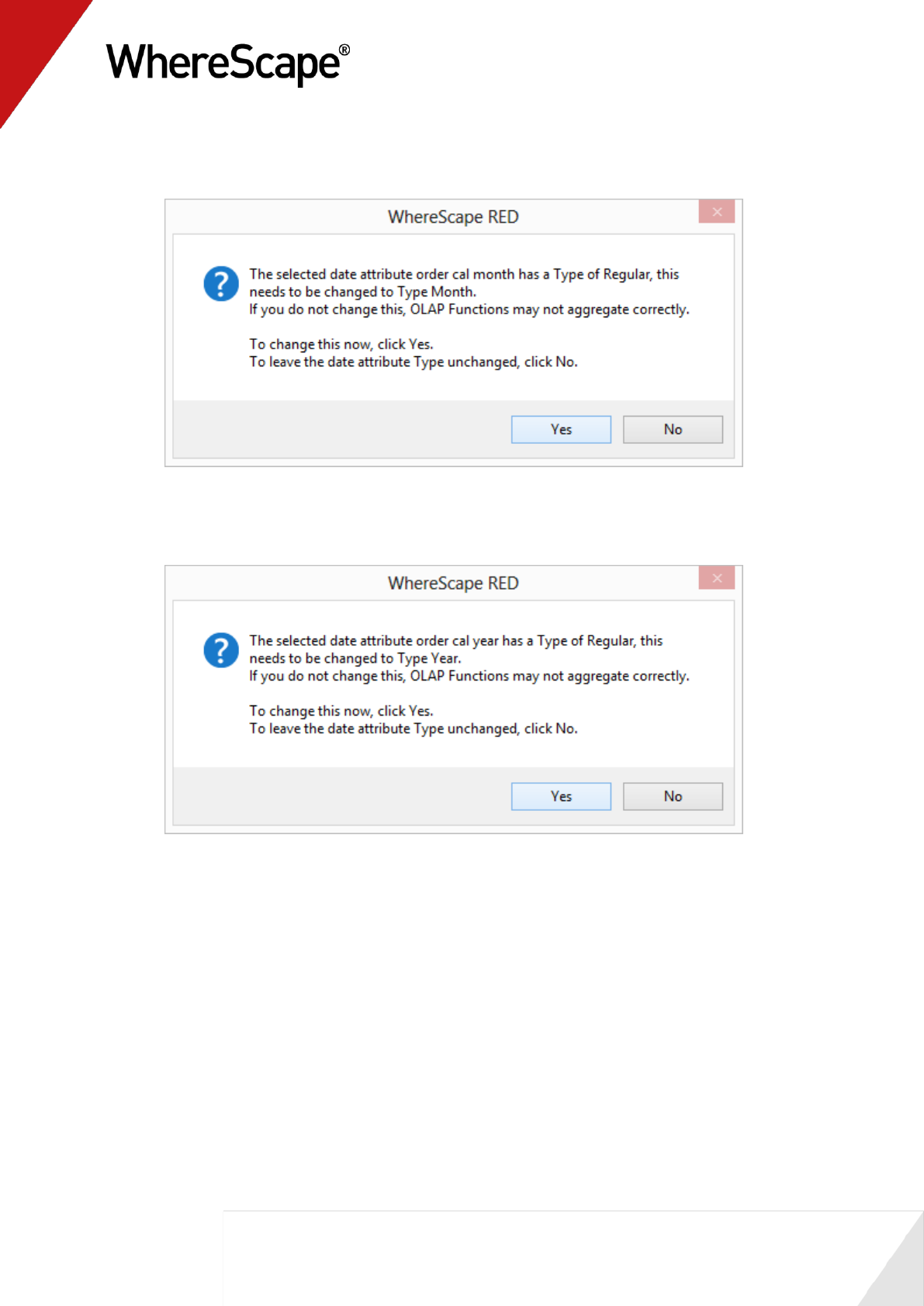
175
11 After selecting the Month level, you will be asked to confirm changing the attribute type to
Months for the the cal month attribute in Analysis Services. Click Yes.
12 Next, for Year Level, select cal year
Similarly, selecting the Year level, you will be asked to confirm changing the attribute
type to Years for the the cal year attribute in Analysis Services. Again click Yes.
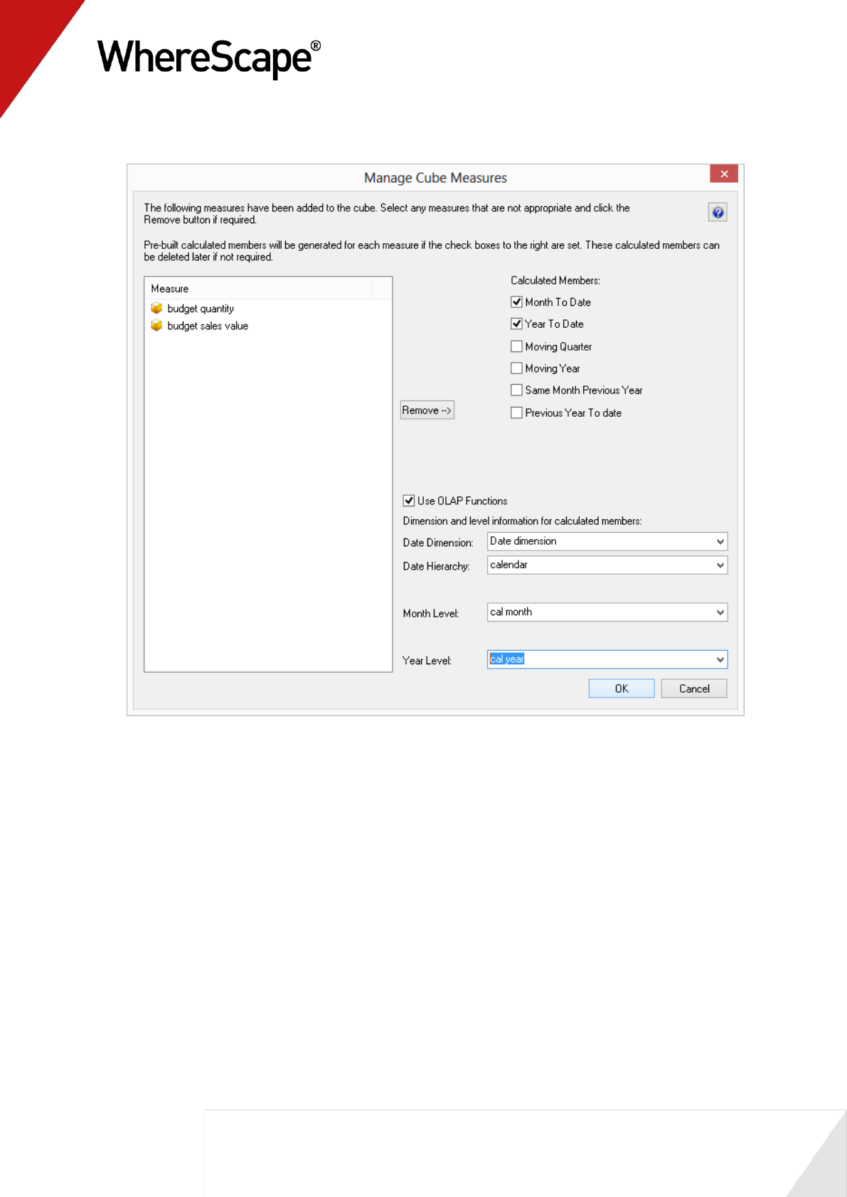
176
13 Your Manage cube measures dialog should now look like this. Click OK.
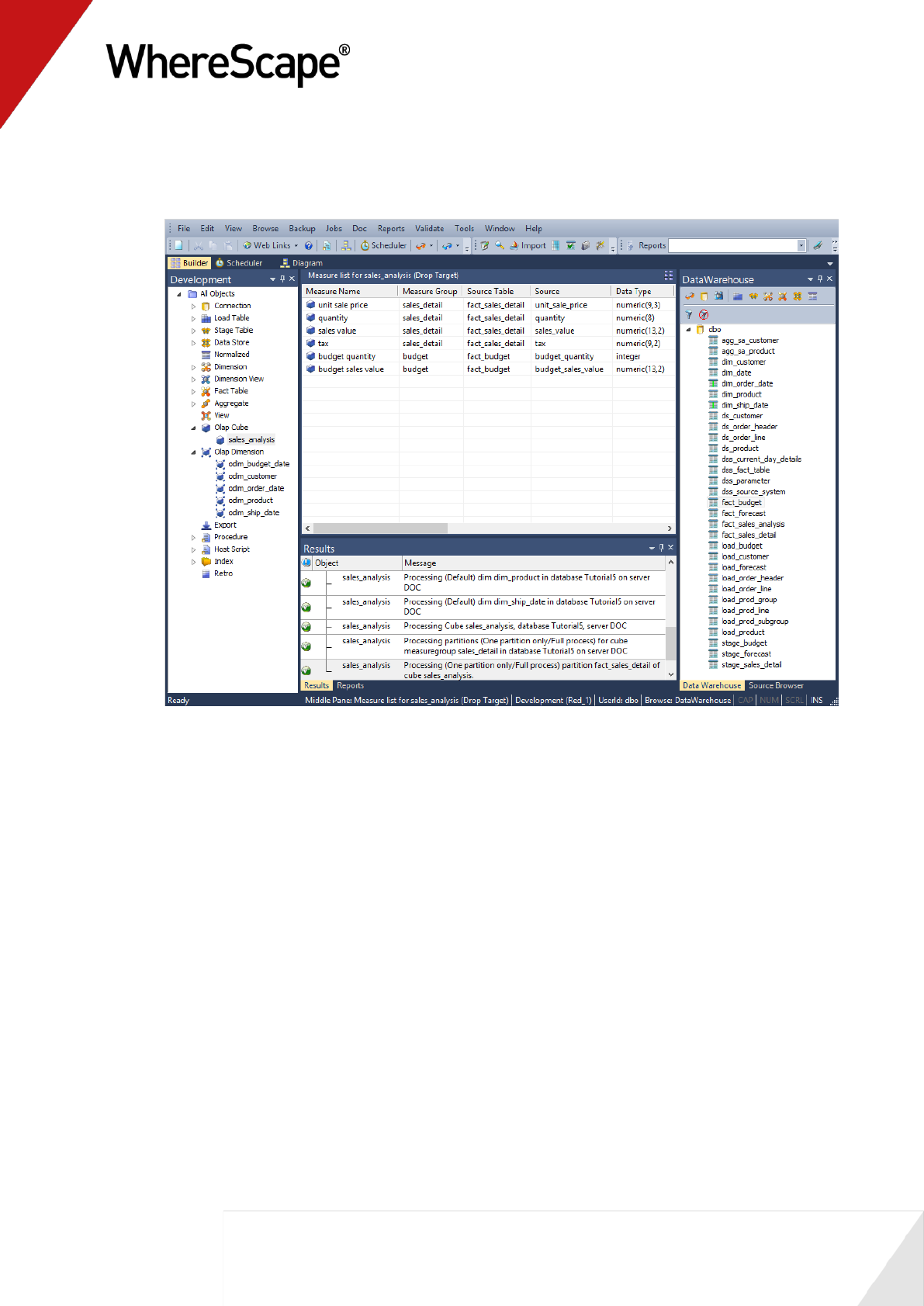
177
14 Click on the OLAP Cube sales_analysis in the left pane to show the updated Measures
associated with the cube.
You should now see measures from both fact tables in the middle pane:
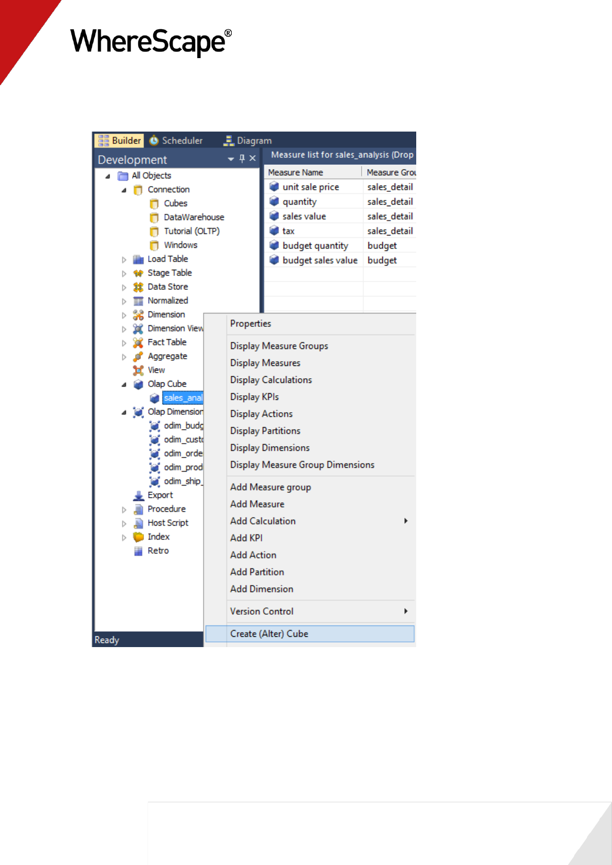
178
15 To apply the changes made in the WhereScape RED metadata to Analysis Services, right-click
on the sales_analysis OLAP Cube in the left pane and select Create (Alter) Cube.
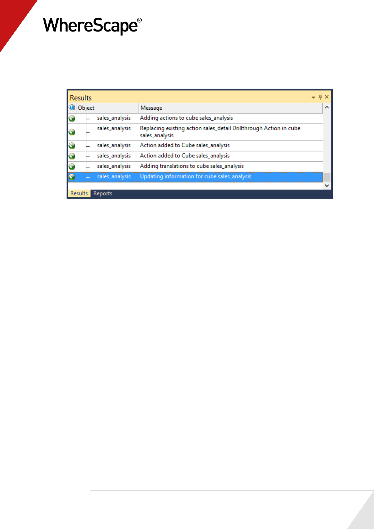
179
16 This will open the WSL Cube executable that connects to Analysis Services to create the
sales_analysis cube structure.
You will see the successful completion in the results pane.

180
17 Next, reload the OLAP Cube in Analysis Services by right-clicking on the sales_analysis cube
in the left pane and choosing Update.
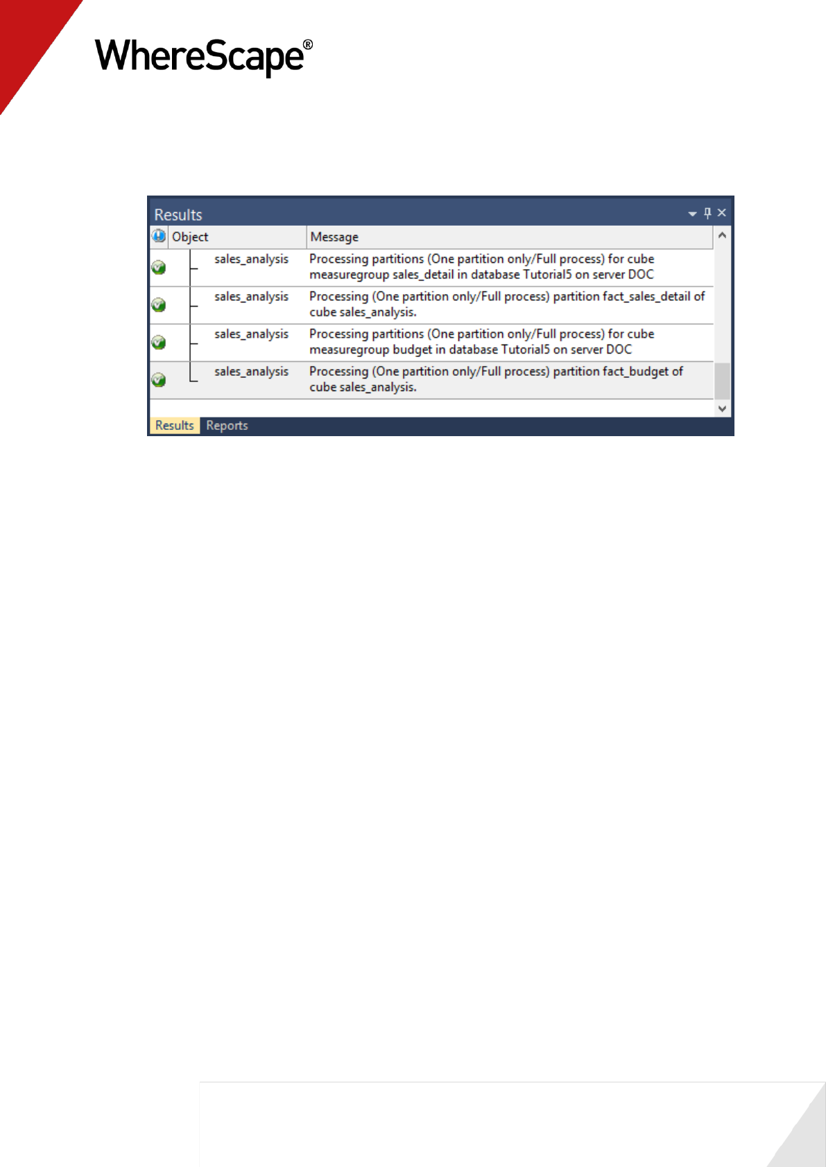
181
18 This will open the OLAP Cube executable to process data into the cube structure. Once the
cube is processed it can be viewed. Again, you will see the successful completion in the
results pane.

182
19 To view the cube in Excel, right-click the sales_analysis cube in the left pane and select
Query cube Via Excel.
20 This will open Excel if it is installed.
Note: If Excel displays a security notice dialog box, click Enable.
However, note that this message may not be displayed.
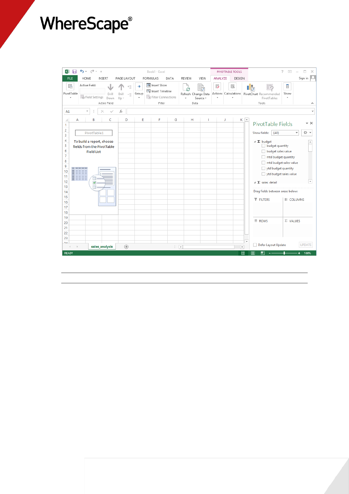
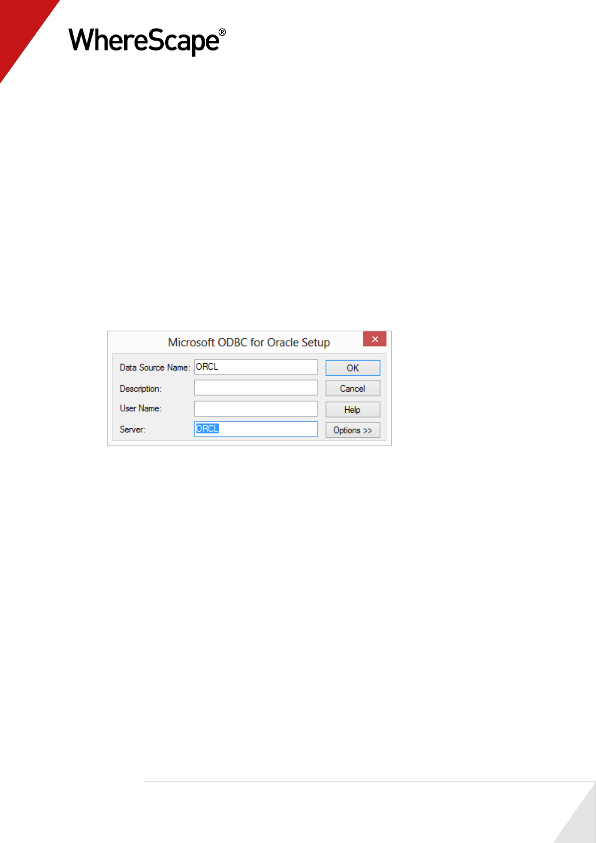
184
5.4 Cube Connections for Other Databases
This tutorial has been completed using Microsoft SQL Server as the data warehouse database. If
you wish to use Oracle or DB2, the data warehouse connections need to be set differently as
follows.
This section shows how to configure the DataWarehouse connection for either an Oracle or a DB2
data warehouse database.
Oracle Configuration
1 Select MSDAORA for the Connection Provider/Driver
Enter the oracle TNS Server Name for the Data Warehouse Server, specifically the
Server field in the ODBC set up screen as in the screenshot below:

185
2 Enter the data warehouse "schema" for the Data Warehouse Database ID field.
Here is an Oracle example:
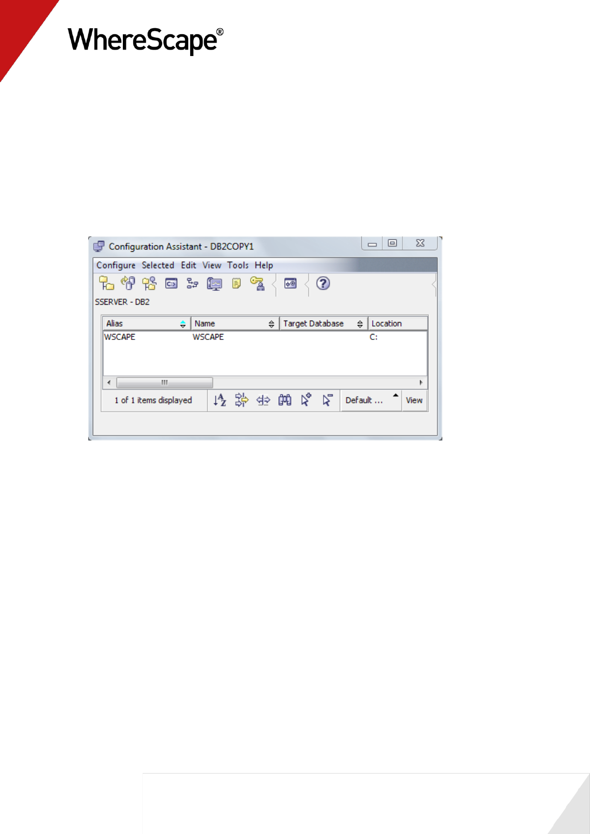
186
DB2 Configuration
1 Select IBMDADB2 for the Connection Provider/Driver
The Data Warehouse Server field is left empty for DB2
Enter the database server alias for the Data Warehouse Database ID field, specifically
the alias field for the IBM DB2 connection in the following DB2 Configuration Assistant
screen:
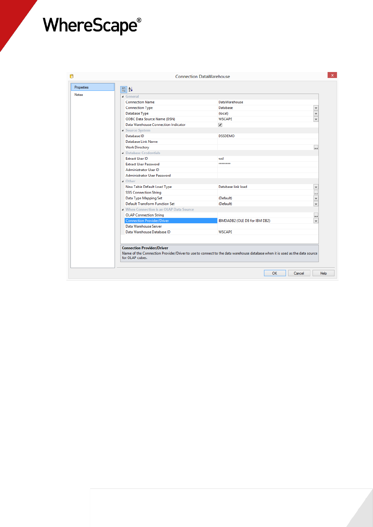
187
2 Here is an IBM DB2 example:
